Buy-Side, Sell-Side, Prop and HFT Firms

Stand at the top of the order book and every trade looks the same: a buy meets a sell, a price prints, the tape ticks on. But the people on the other side of your fills are not one crowd. They are four quite different businesses, each making money in a fundamentally different way, each pointing its quants at a different problem. A long-only fund manager, a bank's execution desk, a proprietary trading shop and a high-frequency market maker can all touch the same RELIANCE order in the same second, yet they want completely different things from it. Knowing who is who - and which one you are - is the first map a quant needs.

The four businesses sharing one order book

Buy-side firms manage other people's money and charge for the privilege. In India this is the world of AMCs (asset management companies, which run mutual funds), PMS (portfolio management services, with a high minimum ticket set by SEBI, currently Rs 50 lakh), and AIFs (alternative investment funds, whose Category III is the closest thing India has to a classic hedge fund and can short and use leverage within limits). Their raw material is alpha - return above a benchmark - and their revenue is fees charged on AUM (assets under management), sometimes with a performance cut on top. A buy-side quant's job is to find holdings that beat the index and to do it at a size that can absorb real money.

Sell-side firms - banks and brokers - mostly do not take large directional bets. They are the plumbing: they provide market access, execution, research, financing and, for the largest, liquidity provision. They are paid per unit of flow - commission and, where they make markets, the bid-ask spread. A sell-side quant lives in execution algorithms, order routing and risk on inventory, not in long-horizon stock picking.

Prop (proprietary) shops trade their own capital. No clients, no management fees, no AUM to gather - they keep every rupee of profit and eat every rupee of loss. Their edge is the model itself and the speed of getting it to market. HFT (high-frequency trading) houses are a specialised prop subset that competes on latency: they quote both sides of the book as market makers, capture the spread thousands of times a day, and run latency and statistical arbitrage measured in microseconds.

These four are not abstractions. They operate in a genuinely enormous pool of money, and it helps to feel the scale before we talk strategy:

# The rupee scale of the arena: average daily traded value of a few heavyweight names.
import os
from datetime import datetime, timedelta

from openalgo import api

client = api(
    api_key=os.getenv("OPENALGO_API_KEY", "your_api_key_here"),
    host=os.getenv("OPENALGO_HOST", "http://127.0.0.1:5000"),
)

end = datetime.now().strftime("%Y-%m-%d")
start = (datetime.now() - timedelta(days=400)).strftime("%Y-%m-%d")
basket = ["RELIANCE", "HDFCBANK", "ICICIBANK", "SBIN", "TCS", "INFY"]

total_cr = 0.0
print("Average daily traded value over the last year (close x volume):")
for sym in basket:
    df = client.history(symbol=sym, exchange="NSE", interval="D",
                        start_date=start, end_date=end).tail(250)
    adtv_cr = (df["close"] * df["volume"]).mean() / 1e7  # rupees -> crore
    total_cr += adtv_cr
    print(f"  {sym:<10} Rs {adtv_cr:8.0f} crore/day")

print(f"\nJust {len(basket)} names turn over about Rs {total_cr:,.0f} crore every single day.")
print("This is the rupee ocean that buy-side, sell-side, prop and HFT desks all swim in.")

Average daily traded value over the last year (close x volume):
  RELIANCE   Rs     1888 crore/day
  HDFCBANK   Rs     2470 crore/day
  ICICIBANK  Rs     1796 crore/day
  SBIN       Rs     1218 crore/day
  TCS        Rs      989 crore/day
  INFY       Rs     1430 crore/day

Just 6 names turn over about Rs 9,792 crore every single day.
This is the rupee ocean that buy-side, sell-side, prop and HFT desks all swim in.

Six names - RELIANCE, HDFCBANK, ICICIBANK, SBIN, TCS and INFY - turn over roughly Rs 9,792 crore every single day between them, with HDFCBANK alone near Rs 2,470 crore. The whole cash market is many multiples of that, and the derivatives segment dwarfs the cash market again. This is the ocean all four businesses swim in. The point is not the exact figure, which moves daily, but the order of magnitude: there is more than enough liquidity here for very different players to coexist.

Follow the money: how incentives shape the quant work

Once you know how a firm gets paid, you can predict what its researchers care about, because the revenue model and the research problem are the same thing seen from two sides.

A fee-on-AUM business is rewarded for gathering and keeping assets, so its quants optimise risk-adjusted return at capacity. A strategy that earns a beautiful Sharpe ratio on Rs 1 crore but chokes at Rs 500 crore is nearly useless to a large AMC, because it cannot move the needle on the fees. Drawdown control matters intensely too - investors redeem after pain, and redemptions are the real enemy. So buy-side quants lean toward lower turnover, longer horizons, broad diversification and capacity (a theme we develop in chapter 48).

A spread-and-commission business is rewarded per unit of flow, so its quants optimise execution quality and inventory. The questions are microstructural: what is my fill rate, how much am I paying to cross the spread, what is my order-to-trade ratio, how do I unwind inventory without moving the price against myself. This is the entire subject of Module C, and the market-making and order-to-trade material in chapters 35 and 38.

An own-P&L business keeps everything it makes, so its quants are merciless about net edge after costs. There is no management fee to cushion a mediocre year. For a prop desk the binding constraints are the per-trade edge and, for HFT, the latency arms race - colocation, dedicated lines, sometimes custom hardware. The economics are unforgiving: if your average edge per trade is smaller than your average cost per trade, more volume just loses money faster.

The holding-period spectrum

The cleanest way to tell these firms apart is not their letterhead but their clock. How long do they hold a position, and therefore how often do they trade? Turnover - the rate at which a book flips its positions - is the single fingerprint that places a firm on the map, and it is something you can measure directly from a strategy:

Copy

# The holding-period spectrum: how often three styles flip position per year on NIFTY.
import os
from datetime import datetime
from pathlib import Path

import matplotlib

matplotlib.use("Agg")
import matplotlib.pyplot as plt
import numpy as np
import seaborn as sns
from openalgo import api, ta

client = api(
    api_key=os.getenv("OPENALGO_API_KEY", "your_api_key_here"),
    host=os.getenv("OPENALGO_HOST", "http://127.0.0.1:5000"),
)

end = datetime.now().strftime("%Y-%m-%d")
df = client.history(symbol="NIFTY", exchange="NSE_INDEX", interval="D",
                    start_date="2021-01-01", end_date=end)
c = df["close"]
years = len(c) / 252.0

# Three position rules, fast to slow.
fast = np.sign(c.pct_change()).fillna(0)                       # flip with daily direction (prop/HFT proxy)
medium = np.where(ta.sma(c, 20) > ta.sma(c, 100), 1.0, -1.0)   # 20/100 SMA trend (systematic fund)
medium = np.nan_to_num(medium)
hold = np.ones(len(c))                                         # buy-and-hold (long-only investor)

def flips_per_year(pos):
    pos = np.asarray(pos, dtype=float)
    return int((np.diff(pos) != 0).sum()) / years

styles = {"Prop / HFT\n(daily flip)": flips_per_year(fast),
          "Systematic fund\n(20/100 trend)": flips_per_year(medium),
          "Long-only investor\n(buy & hold)": flips_per_year(hold)}

sns.set_theme(style="whitegrid")
fig, ax = plt.subplots(figsize=(8, 5))
bars = ax.bar(list(styles), list(styles.values()),
              color=["#dc2626", "#7c83ff", "#16a34a"])
ax.set_yscale("symlog")
ax.set_ylabel("Position flips per year (turnover)")
ax.set_title(f"NIFTY {c.index[0].date()} to {c.index[-1].date()}: the holding-period spectrum")
for b, v in zip(bars, styles.values()):
    ax.text(b.get_x() + b.get_width() / 2, v + 0.3, f"{v:.0f}/yr", ha="center", fontweight="600")

out = Path(__file__).with_suffix(".png")
plt.savefig(out, dpi=110, bbox_inches="tight")
f_fast, f_trend, f_hold = list(styles.values())
print(f"{len(c)} NIFTY days ({years:.1f} yrs). Flips/yr -> "
      f"fast {f_fast:.0f}, trend {f_trend:.0f}, hold {f_hold:.0f}. Saved {out.name}")

Live output

1358 NIFTY days (5.4 yrs). Flips/yr -> fast 113, trend 3, hold 0. Saved 02_turnover_spectrum.png

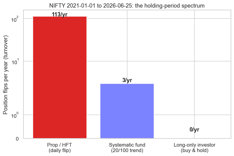
Run on 5.4 years of NIFTY, three position rules sit at three very different points on the spectrum. A fast rule that flips with each day's direction trades about 113 times a year - a daily proxy for the prop and HFT end, where the real article flips thousands of times a day. A 20/100 moving-average trend, the kind of medium-horizon signal a systematic fund might run, flips only about 3 times a year. And buy-and-hold flips zero times - the long-only investor simply owns the market. Same instrument, same five years, turnover spanning two orders of magnitude.

Turnover is not a vanity metric - it dictates how sensitive a strategy is to cost. A book that flips 113 times a year pays the bid-ask spread and exchange charges 113 times; one that flips three times a year pays it three times. This is why the same raw signal can be a winner for a slow fund and a loser for a fast desk, and why every honest backtest has to be run net of realistic costs (the trap we hammer in Module H). High turnover is only viable when the edge captured per trade comfortably exceeds the cost paid per trade - which is exactly why HFT obsesses over both spread capture and latency, and why a long-only AMC barely thinks about microstructure at all.

Where a retail quant actually fits

Here is the honest placement. You will not win the microsecond war; that ground belongs to well-capitalised HFT houses and is defended with infrastructure you cannot match. But the medium-horizon, systematic space - holding days to weeks, trading a handful to a few dozen times a month - is genuinely open. At small size, the capacity constraint that haunts a large AMC is your friend: you can hold positions a Rs 5,000 crore fund cannot, because you are not trying to move Rs 500 crore through a thin order book.

The four businesses are not rivals so much as a food chain. Buy-side capital supplies the slow, large orders. Market makers and HFT supply the liquidity those orders consume, earning the spread in return. Sell-side desks connect the two and clip a fee for the introduction. Prop desks hunt the inefficiencies left in the gaps. Each needs the others, and price is simply where their incentives meet. In the next chapter we zoom into who actually moves prices on a given day - retail, HNI, foreign and domestic institutions, prop and market makers - and how to read their footprints in the data.