Statistical Arbitrage

Now we build our first real strategy, and it's the purest one in quant finance: an edge that doesn't care whether the market crashes or soars. Statistical arbitrage trades relationships between assets - profiting when a stretched spread snaps back - while being almost perfectly indifferent to the market's direction. Chapter 17 gave us the mathematics of cointegration; this chapter turns it into a backtested, market-neutral machine, and shows why even a modest return from it can be worth more than a flashy one.

From one pair to a strategy

Recall the cointegrated Reliance-ONGC spread: two energy giants leashed together, their spread mean-reverting around a z-score. The trade wrote itself - short the spread when it's stretched high, buy it when stretched low, exit at fair value. Now let's actually backtest it: simulate the rule over years of history with a rolling z-score (so there's no look-ahead), and see what it would have made.

# Backtest a market-neutral pairs trade on the cointegrated Reliance-ONGC spread.
import os
from datetime import datetime

import numpy as np
import pandas as pd
import statsmodels.api as sm
from openalgo import api

client = api(
    api_key=os.getenv("OPENALGO_API_KEY", "your_api_key_here"),
    host=os.getenv("OPENALGO_HOST", "http://127.0.0.1:5000"),
)

end = datetime.now().strftime("%Y-%m-%d")


def close(sym):
    return client.history(symbol=sym, exchange="NSE", interval="D",
                          start_date="2021-01-01", end_date=end)["close"]


df = pd.concat([close("RELIANCE"), close("ONGC")], axis=1).dropna()
df.columns = ["a", "b"]
hedge = sm.OLS(df["a"], sm.add_constant(df["b"])).fit().params.iloc[1]
spread = df["a"] - hedge * df["b"]
z = (spread - spread.rolling(60).mean()) / spread.rolling(60).std()    # rolling, no look-ahead

# Stateful rule: short spread above +2, long below -2, flat inside +/-0.5.
pos, p = [], 0
for zi in z:
    if not np.isnan(zi):
        if p == 0 and zi > 2:
            p = -1
        elif p == 0 and zi < -2:
            p = 1
        elif p != 0 and abs(zi) < 0.5:
            p = 0
    pos.append(p)
pos = pd.Series(pos, index=z.index)

pnl = (pos.shift(1) * spread.diff()).dropna()
sharpe = pnl.mean() / pnl.std() * np.sqrt(252)
corr = pnl.reindex(df.index).fillna(0).corr(df["a"].pct_change().fillna(0))

print(f"Trades taken        : {(pos.diff().abs() > 0).sum()}")
print(f"Total spread P&L     : {pnl.sum():.0f} points")
print(f"Strategy Sharpe      : {sharpe:.2f}")
print(f"Correlation to market: {corr:+.2f}   (near zero = market-neutral)")
print("\nProfit comes from the spread reverting - not from the market going up or down.")

Trades taken        : 46
Total spread P&L     : 446 points
Strategy Sharpe      : 0.47
Correlation to market: +0.00   (near zero = market-neutral)

Profit comes from the spread reverting - not from the market going up or down.

Forty-six trades, a positive spread P&L, a Sharpe of 0.47 - and the number that matters most: a correlation to the market of 0.00. The strategy made its money purely from the spread reverting, with zero dependence on whether Nifty went up or down. That's not a rounding accident; it's the whole point.

Market-neutral by construction

Why is it market-neutral? Because of how it's built - long one leg, short the other, in the hedge ratio that cancels their shared market exposure:

When the whole market rises, your long leg gains and your short leg loses by almost the same amount - they cancel. What's left is the movement of the spread, which is what you're actually betting on. The construction itself strips out market risk, leaving a pure bet on the relationship.

The equity curve ignores the market

See the independence directly - the pairs P&L plotted against Nifty:

Copy

# The pairs-trade equity curve - market-neutral gains that ignore the index.
import os
from datetime import datetime
from pathlib import Path

import matplotlib

matplotlib.use("Agg")
import matplotlib.pyplot as plt
import numpy as np
import pandas as pd
import seaborn as sns
import statsmodels.api as sm
from openalgo import api

client = api(
    api_key=os.getenv("OPENALGO_API_KEY", "your_api_key_here"),
    host=os.getenv("OPENALGO_HOST", "http://127.0.0.1:5000"),
)

end = datetime.now().strftime("%Y-%m-%d")


def close(sym, exch="NSE"):
    return client.history(symbol=sym, exchange=exch, interval="D",
                          start_date="2021-01-01", end_date=end)["close"]


df = pd.concat([close("RELIANCE"), close("ONGC")], axis=1).dropna()
df.columns = ["a", "b"]
hedge = sm.OLS(df["a"], sm.add_constant(df["b"])).fit().params.iloc[1]
spread = df["a"] - hedge * df["b"]
z = (spread - spread.rolling(60).mean()) / spread.rolling(60).std()

pos, p = [], 0
for zi in z:
    if not np.isnan(zi):
        if p == 0 and zi > 2:
            p = -1
        elif p == 0 and zi < -2:
            p = 1
        elif p != 0 and abs(zi) < 0.5:
            p = 0
    pos.append(p)
pos = pd.Series(pos, index=z.index)
equity = (pos.shift(1) * spread.diff()).fillna(0).cumsum()

nifty = close("NIFTY", "NSE_INDEX")
nifty_norm = (nifty / nifty.iloc[0] - 1) * 100

sns.set_theme(style="whitegrid")
fig, ax1 = plt.subplots(figsize=(8, 4.5))
ax1.plot(equity.index, equity, color="#16a34a", lw=1.8, label="pairs P&L (points)")
ax1.set_ylabel("Pairs P&L (spread points)", color="#16a34a")
ax2 = ax1.twinx()
ax2.plot(nifty_norm.index, nifty_norm, color="#888", lw=1.2, ls="--", label="NIFTY %")
ax2.set_ylabel("NIFTY return %", color="#888")
ax2.grid(False)
ax1.set_title("Reliance-ONGC pairs trade vs the market - notice they don't move together")
out = Path(__file__).with_suffix(".png")
plt.savefig(out, dpi=110, bbox_inches="tight")
print(f"Pairs P&L {equity.iloc[-1]:.0f} points, while NIFTY did {nifty_norm.iloc[-1]:+.0f}%. Saved {out.name}")

Live output

Pairs P&L 446 points, while NIFTY did +71%. Saved 02_pairs_equity.png

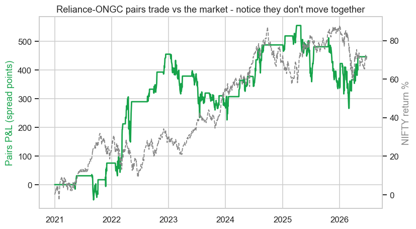
While Nifty rallied +71% over the window, the pairs trade ground out its own modest P&L on a completely different rhythm - rising when the market fell, flat when the market soared, marching to the spread's drum, not the index's. A line that ignores the market is exactly what a diversified book craves.

Why a modest Sharpe is still gold

A standalone Sharpe of 0.47 sounds unexciting next to a trend-follower's flashier numbers. But that misses the magic. A zero-correlation return stream is worth far more than its solo Sharpe suggests, because when you add it to a portfolio it diversifies everything else (Chapter 23). Run dozens of uncorrelated pairs at once and their individual noise averages out while their small edges accumulate - producing a smooth, market-independent equity curve that's the envy of every directional trader. Statistical arbitrage is a team sport: no single pair is the strategy; the diversified ensemble is.

Beyond pairs: baskets, index and cash-futures

The same idea scales up across India's market:

• Basket / index arbitrage - trade an index against a basket of its constituents (or its future), capturing tiny dislocations between the whole and its parts.
• Cash-futures arbitrage - the desk staple from Chapter 19: when the future's basis strays from fair carry, buy the cheap one and sell the dear one, locking the convergence. It's low-risk, capacity-heavy, and runs on nearly every Indian prop desk.

All are the same DNA: identify a relationship that must hold by no-arbitrage or cointegration, trade its temporary deviations, stay market-neutral.

Try it yourself

• Run the backtest with tighter entry bands (z > 1.5 instead of 2). More trades, but is the Sharpe higher or lower after the extra costs?
• Add a second cointegrated pair and combine the two P&L streams. Is the blended Sharpe higher than either alone? (That's the diversification magic.)
• Add a stop: exit if the z-score keeps widening past 3.5 (the leash may have snapped). Does it protect against the worst losses?

Recap

• Statistical arbitrage trades mean-reverting relationships, profiting from a stretched spread snapping back - indifferent to market direction.
• Backtested, the Reliance-ONGC pairs trade was market-neutral (correlation 0.00) - its P&L ignored Nifty's +71% rally entirely.
• It's neutral by construction: long one leg, short the other, so shared market moves cancel and only the spread remains.
• A modest standalone Sharpe (0.47) is gold when it's uncorrelated - diversify across many pairs and the ensemble is smooth and market-independent.
• The idea scales to basket, index and cash-futures arbitrage - but watch for broken cointegration, crowding and thin-spread costs.

Stat-arb was market-neutral and relationship-driven. The next strategy family takes a directional view, but a disciplined, systematic one - cross-sectional momentum and value, the workhorses of quant equity.