Optimization, Constraints and Numerical Methods

Almost every quant model, once you strip away the story, ends in the same sentence: find the inputs that make this one number as good as possible. Find the weights that give the lowest-risk portfolio. Find the parameters that fit the volatility surface tightest. Find the trade schedule that costs the least to execute. That hunt for the best inputs is optimization, and it is the quiet engine sitting under portfolio construction, model calibration, and execution. This chapter is the toolbox: what you are minimising, why the shape of the problem decides whether you can trust the answer, and the numerical traps that turn a clean formula into garbage. It closes the mathematics module and hands you the exact machinery Chapter 72 uses to build a portfolio.

The objective function

Optimization needs a single number to chase. That number comes from an objective function (also called a loss or cost function): a function that takes your choices and returns one scalar measuring how good or bad they are. Minimise it, or maximise it - the two are the same problem with a sign flip. For a portfolio, the classic objective is variance, written w' Σ w, where w is the vector of weights and Σ is the covariance matrix of returns we met in Chapter 15. Feed in a set of weights, get back a single number for the portfolio's risk. The whole job is to find the w that makes it smallest.

Picture the objective as a landscape. Each choice of inputs is a location, the objective's value is the altitude, and we are a ball trying to roll to the lowest valley. That mental picture - a surface with hills and basins - is worth holding onto, because the terrain is what separates an easy problem from a hopeless one.

Convex versus non-convex

The single most important question about any optimization is whether it is convex. A convex problem has a landscape shaped like one clean bowl: wherever you drop the ball, it rolls to the same bottom, and that bottom is the true, global best. There are no false valleys to get stuck in. Portfolio variance is convex (because a covariance matrix is positive semi-definite), which is a gift - it means the minimum-variance portfolio is unique and a solver will actually find it.

A non-convex problem is the nightmare twin: a landscape of many basins, ridges and false bottoms. The ball rolls into whichever local minimum is nearest, and you have no guarantee it is the global minimum you wanted. Calibrating a complex model, fitting a neural network, or optimising a path-dependent strategy is usually non-convex, and there you must accept that the answer depends on where you started.

How a solver descends

Given a smooth objective, how does the solver actually get to the bottom? Two ideas underpin almost everything. Gradient descent reads the slope (the gradient) at the current point and takes a step downhill, the direction of steepest descent, then repeats. It only needs first derivatives, so it scales to huge problems, but it can crawl and zig-zag through narrow valleys. Newton's method is the smarter, greedier cousin: it also uses the curvature (the second derivative, or Hessian) to jump in one move close to where the bowl bottoms out. Newton converges in far fewer steps when it works, but it needs the Hessian and can misbehave far from the minimum. Most production solvers blend the two - using curvature where it helps, falling back to safe gradient steps where it does not.

Adding constraints

An unconstrained minimum is often useless in finance. A pure minimum-variance solver, left free, will happily short some names heavily and lever others past 100%. Real mandates forbid that, so we impose constraints: equalities like "the weights must sum to one" (the budget constraint) and inequalities like "no weight may be negative" (long-only) or "no name above 10%". Constraints carve a feasible region out of the landscape - the set of allowed choices - and the solver must find the lowest point inside that region.

This changes the answer in a specific way. If the free minimum already sits inside the feasible region, the constraints do nothing. But if it sits outside, the constrained optimum gets pushed to the boundary - it sits exactly on a constraint, as the purple dot does in the figure above. The mathematics that describes which constraints are "binding" like this is the Karush-Kuhn-Tucker (KKT) conditions, the constrained generalisation of "set the derivative to zero". You rarely solve KKT by hand, but the intuition is everything: a constraint that binds always costs you something on the objective, because it stops the ball reaching the true bottom.

Quadratic programming for portfolios

When the objective is quadratic (like w' Σ w) and the constraints are linear (weights sum to one, weights non-negative), the problem has a name: a quadratic program (QP). This is the workhorse of portfolio construction, because Markowitz mean-variance optimization is exactly a QP, and it is convex, so it solves fast and uniquely. Let us actually solve one on real data.

# Minimum-variance portfolio on 5 real Nifty stocks: the quadratic program quants solve.
import os
from datetime import datetime

import numpy as np
from openalgo import api
from scipy.optimize import minimize

client = api(
    api_key=os.getenv("OPENALGO_API_KEY", "your_api_key_here"),
    host=os.getenv("OPENALGO_HOST", "http://127.0.0.1:5000"),
)

stocks = ["RELIANCE", "HDFCBANK", "INFY", "ITC", "SBIN"]
end = datetime.now().strftime("%Y-%m-%d")

# Build the daily log-return matrix (one column per stock).
cols = {}
for s in stocks:
    px = client.history(symbol=s, exchange="NSE", interval="D",
                        start_date="2023-01-01", end_date=end)["close"]
    cols[s] = np.log(px / px.shift(1))
import pandas as pd
R = pd.DataFrame(cols).dropna()

# Annualised covariance matrix - the Sigma in w' Sigma w.
Sigma = R.cov().values * 252
n = len(stocks)


def port_vol(w):
    return np.sqrt(w @ Sigma @ w)


# Long-only minimum-variance: minimise w' Sigma w s.t. sum(w)=1, w>=0.
cons = ({"type": "eq", "fun": lambda w: w.sum() - 1.0},)
bounds = [(0.0, 1.0)] * n
res = minimize(port_vol, np.repeat(1.0 / n, n), method="SLSQP",
               bounds=bounds, constraints=cons)
w = res.x

# Closed-form (unconstrained) check: w = Sig^-1 1 / (1' Sig^-1 1).
inv1 = np.linalg.solve(Sigma, np.ones(n))
w_cf = inv1 / inv1.sum()

print("Minimum-variance weights (long-only QP):")
for s, wi in zip(stocks, w):
    print(f"  {s:9s} {wi:6.1%}")
print(f"\nPortfolio volatility   : {port_vol(w):.2%} per year")
print(f"Equal-weight volatility: {port_vol(np.repeat(1/n, n)):.2%} per year")
print(f"Closed-form min-var vol : {port_vol(w_cf):.2%}  "
      f"(weights {', '.join(f'{x:.0%}' for x in w_cf)})")
print(f"\n{len(R)} trading days, {n} stocks. Optimiser converged: {res.success}")

Minimum-variance weights (long-only QP):
  RELIANCE   14.2%
  HDFCBANK   25.2%
  INFY       16.8%
  ITC        35.1%
  SBIN        8.7%

Portfolio volatility   : 13.33% per year
Equal-weight volatility: 13.87% per year
Closed-form min-var vol : 13.33%  (weights 14%, 25%, 17%, 35%, 9%)

861 trading days, 5 stocks. Optimiser converged: True

Over 861 trading days of five real Nifty names, the long-only minimum-variance portfolio lands on RELIANCE 14.2%, HDFCBANK 25.2%, INFY 16.8%, ITC 35.1% and SBIN 8.7%, for an annualised volatility of 13.33% - meaningfully below the equal-weight portfolio's 13.87%. That is the whole promise of diversification, made numerical. Notice too that the closed-form solution Σ⁻¹1 / 1'Σ⁻¹1 gives the same 13.33%: here the unconstrained optimum is already long-only, so the non-negativity constraint never binds. When it does bind - when the free solution wants to short something - the QP and the closed form part ways, and only the QP respects the mandate.

The efficient frontier

The minimum-variance portfolio is one point. Sweep the constraint "achieve at least this expected return" across a range of targets and re-solve each time, and you trace the efficient frontier: the set of portfolios giving the least risk for each level of return. Every rational long-only portfolio of these assets lives on or inside this curve.

Copy

# The efficient frontier from 5 real Nifty stocks, with the minimum-variance point marked.
import os
from datetime import datetime
from pathlib import Path

import matplotlib

matplotlib.use("Agg")
import matplotlib.pyplot as plt
import numpy as np
import pandas as pd
import seaborn as sns
from openalgo import api
from scipy.optimize import minimize

client = api(
    api_key=os.getenv("OPENALGO_API_KEY", "your_api_key_here"),
    host=os.getenv("OPENALGO_HOST", "http://127.0.0.1:5000"),
)

stocks = ["RELIANCE", "HDFCBANK", "INFY", "ITC", "SBIN"]
end = datetime.now().strftime("%Y-%m-%d")

cols = {}
for s in stocks:
    px = client.history(symbol=s, exchange="NSE", interval="D",
                        start_date="2023-01-01", end_date=end)["close"]
    cols[s] = np.log(px / px.shift(1))
R = pd.DataFrame(cols).dropna()

mu = R.mean().values * 252          # annualised expected returns
Sigma = R.cov().values * 252        # annualised covariance
n = len(stocks)


def vol(w):
    return np.sqrt(w @ Sigma @ w)


def frontier_point(target):
    cons = ({"type": "eq", "fun": lambda w: w.sum() - 1.0},
            {"type": "eq", "fun": lambda w: w @ mu - target})
    res = minimize(vol, np.repeat(1 / n, n), method="SLSQP",
                   bounds=[(0, 1)] * n, constraints=cons)
    return res.x

# Minimum-variance portfolio (no return target).
mv = minimize(vol, np.repeat(1 / n, n), method="SLSQP",
              bounds=[(0, 1)] * n,
              constraints=({"type": "eq", "fun": lambda w: w.sum() - 1.0},)).x

targets = np.linspace(mu.min(), mu.max(), 40)
fvol = [vol(frontier_point(t)) for t in targets]

sns.set_theme(style="whitegrid")
fig, ax = plt.subplots(figsize=(8.5, 5.5))
ax.plot(fvol, targets, color="#7c83ff", lw=2.2, label="Efficient frontier")
ax.scatter(np.sqrt(np.diag(Sigma)), mu, color="#dc2626", s=55, zorder=5)
for s, v, m in zip(stocks, np.sqrt(np.diag(Sigma)), mu):
    ax.annotate(s, (v, m), textcoords="offset points", xytext=(7, 2), fontsize=9)
ax.scatter([vol(mv)], [mv @ mu], color="#16a34a", s=130, marker="*",
           zorder=6, label="Minimum variance")
ax.set_xlabel("Annualised volatility")
ax.set_ylabel("Annualised expected return")
ax.set_title("Efficient frontier - 5 Nifty stocks (2023-present)")
ax.legend()
out = Path(__file__).with_suffix(".png")
plt.savefig(out, dpi=110, bbox_inches="tight")
print(f"Min-variance point: vol {vol(mv):.2%}, return {mv @ mu:.2%}. "
      f"Frontier spans vol {min(fvol):.2%}-{max(fvol):.2%}. Saved {out.name}")

Live output

Min-variance point: vol 13.33%, return 0.29%. Frontier spans vol 13.33%-25.52%. Saved 02_efficient_frontier.png

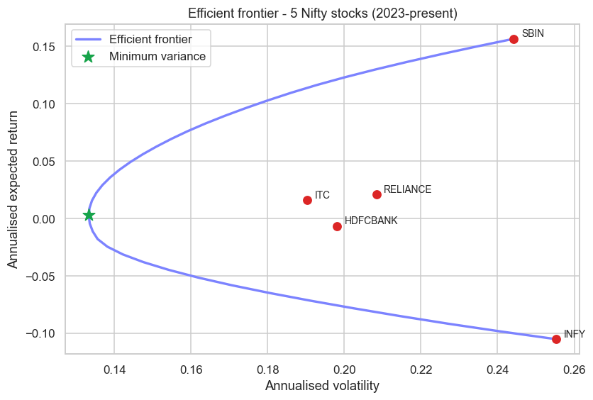
The curve spans annualised volatility from 13.33% at the minimum-variance tip out to 25.52%, with the green star marking that lowest-risk corner. But look closely and you meet a warning, not just a result: the return axis depends on those annualised mean estimates, and over this window INFY's mean is negative while SBIN's is strongly positive. Those means are estimated from a few hundred noisy observations, and they move the frontier around far more than the risk numbers do.

Numerical-stability traps

The same optimization can be rock-solid or wildly unstable depending on the numbers you feed it, and the covariance matrix is where it breaks. If two assets are nearly perfectly correlated, or you estimate a large covariance matrix from too few observations, Σ becomes ill-conditioned: nearly singular, so inverting it amplifies tiny estimation errors into enormous, nonsensical weights. The cure is to condition the inputs before optimising - shrink the covariance matrix toward a simpler target (Ledoit-Wolf), clean its eigenvalues (the PCA view from Chapter 15), or add a small ridge to its diagonal. A few practical guardrails:

• Optimise in sensible units and scale your variables so the objective is not dominated by one huge term.
• Never invert a covariance matrix you estimated from fewer observations than assets - it is rank-deficient by construction.
• Prefer a solver that takes the matrix directly over one that forms Σ⁻¹ explicitly; explicit inverses are numerically fragile.
• Sanity-check the output: if the optimal weights lurch on a tiny data change, your inputs, not your solver, are the problem.

We now have the full mathematical toolkit of Module B: returns and their stylized facts, probability and inference, the random walk, the linear algebra of risk, and now the optimization that turns all of it into decisions. Module C steps back into the real market - microstructure, the order book, and the cost of actually trading - before we put this machinery to work building portfolios in Chapter 72.