The True Cost of a Trade

Every backtest you'll ever run has a silent enemy, and it isn't the market. It's cost. A strategy that looks brilliant on paper can be a steady loser in reality, and the entire difference is the money that leaks out on every single trade - brokerage, taxes, exchange fees, stamp duty. Most beginners wave this away ("brokerage is zero now!"). A quant does the opposite: they model cost first, because cost is the hurdle every edge must clear. Let's measure it exactly.

"Zero brokerage" is not zero cost

Discount brokers reshaped Indian costs around a flat ₹20 per executed order (and free equity delivery), and a generation of traders concluded trading is basically costless. Let's test that on a standard trade - a ₹1,000 instrument, 500 units, bought and sold - across the four segments you'll actually trade, and add up every rupee that leaves your pocket:

# The real all-in cost of a trade under the Rs 20-per-order discount-broker model.
# Many Indian discount brokers follow this: a flat Rs 20 per executed order
# (equity delivery free). Rates are representative - verify the latest circulars.

EQ, OPT = (1000, 500), (100, 500)          # (price, qty): a Rs 1000 stock; a Rs 100 option


def breakdown(price, qty, *, brokerage, stt, exch_rate, stamp_rate):
    side = price * qty                      # value of one leg (buy = sell here)
    turnover = 2 * side
    exch = exch_rate * turnover
    sebi = 0.000001 * turnover              # Rs 10 per crore
    gst = 0.18 * (brokerage + exch + sebi)  # GST on brokerage + exchange + SEBI
    stamp = round(stamp_rate * side)        # on the buy side, to the nearest rupee
    total = brokerage + stt + exch + sebi + gst + stamp
    return total, qty


flat20 = lambda v: min(0.0003 * v, 20)      # Rs 20 or 0.03% per order, whichever is lower
eq_side, opt_side = EQ[0] * EQ[1], OPT[0] * OPT[1]

segments = {
    "Delivery equity": breakdown(*EQ, brokerage=0,                  stt=0.001 * eq_side * 2, exch_rate=0.0000307, stamp_rate=0.00015),
    "Intraday equity": breakdown(*EQ, brokerage=2 * flat20(eq_side), stt=0.00025 * eq_side,  exch_rate=0.0000307, stamp_rate=0.00003),
    "F&O futures":     breakdown(*EQ, brokerage=2 * flat20(eq_side), stt=0.0005 * eq_side,   exch_rate=0.0000183, stamp_rate=0.00002),
    "F&O options":     breakdown(*OPT, brokerage=2 * 20,            stt=0.0015 * opt_side,  exch_rate=0.0003553, stamp_rate=0.00003),
}

print(f"{'SEGMENT':18s}{'ALL-IN COST':>13s}{'BREAKEVEN (pts)':>18s}")
for name, (total, qty) in segments.items():
    print(f"{name:18s}{total:>13.2f}{total / qty:>18.2f}")
print("\nDelivery brokerage is ZERO, yet the trade still costs 1112 - STT alone is the giant.")
print("Flat Rs 20/order barely moves the needle; in India, STT dominates the bill.")

SEGMENT             ALL-IN COST   BREAKEVEN (pts)
Delivery equity         1112.41              2.22
Intraday equity          224.61              0.45
F&O futures              329.97              0.66
F&O options              166.24              0.33

Delivery brokerage is ZERO, yet the trade still costs 1112 - STT alone is the giant.
Flat Rs 20/order barely moves the needle; in India, STT dominates the bill.

Read the delivery row first. Brokerage was genuinely zero - and yet the round trip still cost ₹1,112, a breakeven of 2.22 points before you make a paisa. Where did it go? One charge dwarfs all the rest: STT (Securities Transaction Tax) - ₹1,000 of that ₹1,112. In India, STT is the cost that matters: it's charged on turnover, it's unavoidable, and on delivery it hits both the buy and the sell. And notice the intraday, futures and options rows - even where the flat ₹20 brokerage applies, it's a rounding error next to STT. "Zero brokerage" quietly hid a tax bill many times larger than brokerage ever was.

The cost stack, line by line

Six charges sit on a typical equity trade, and you should know each by name:

• Brokerage - the broker's fee. Under the discount model many Indian brokers now follow, it's zero for delivery and a flat ₹20 per order (or 0.03%, whichever is lower) for intraday and F&O.
• STT - the big one. A government tax on turnover; rates differ by segment (delivery equity, intraday, futures, options each have their own).
• Exchange transaction charges - the exchange's cut, a tiny percentage of turnover.
• SEBI charges - the regulator's sliver, a few rupees per crore.
• Stamp duty - a state tax, charged on the buy side.
• GST - 18%, but only on the charges (brokerage + exchange + SEBI), not on STT or stamp duty.
• DP charges - a flat fee when you sell from your demat (delivery only).

And the shape of that bill is the real lesson - one line towers over the rest:

Why costs compound

A one-off 0.22% sounds harmless. The danger is that a strategy doesn't trade once - it trades again and again, and the cost is paid every time. Watch what that does over a year:

Copy

# Costs compound. How much does trading frequency quietly bleed from a year's returns?
import os
from pathlib import Path

import matplotlib

matplotlib.use("Agg")
import matplotlib.pyplot as plt
import numpy as np
import seaborn as sns
from openalgo import api

client = api(
    api_key=os.getenv("OPENALGO_API_KEY", "your_api_key_here"),
    host=os.getenv("OPENALGO_HOST", "http://127.0.0.1:5000"),
)

price = client.quotes(symbol="RELIANCE", exchange="NSE")["data"]["ltp"]
buy_val = price * 100
turnover = 2 * buy_val

# Delivery-equity stack (zero brokerage): STT dominates, as a % of capital deployed.
exch = 0.0000307 * turnover               # NSE delivery transaction charge
sebi = 0.000001 * turnover                # Rs 10 / crore
gst = 0.18 * (exch + sebi)
total = 0.001 * turnover + exch + sebi + gst + 0.00015 * buy_val
cost_pct = total / buy_val * 100          # cost of one round trip, in % (~0.22%)

trades = np.arange(0, 261, 10)            # round trips per year
drag = trades * cost_pct                  # annual cost drag, in %

sns.set_theme(style="whitegrid")
fig, ax = plt.subplots(figsize=(8, 4.5))
ax.fill_between(trades, drag, color="#7c83ff", alpha=0.25)
ax.plot(trades, drag, color="#7c83ff", lw=2)
ax.axhline(15, color="#dc2626", ls="--", lw=1.4, label="a 'good' 15% gross edge")
ax.set_title(f"Annual cost drag at {cost_pct:.3f}% per round trip")
ax.set_xlabel("Round trips per year")
ax.set_ylabel("Cost drag (% of capital)")
ax.legend()

out = Path(__file__).with_suffix(".png")
plt.savefig(out, dpi=110, bbox_inches="tight")
print(f"Cost per round trip: {cost_pct:.3f}%")
print(f"At 100 trips/year, costs eat {100 * cost_pct:.1f}% of capital. Saved {out.name}")

Live output

Cost per round trip: 0.222%
At 100 trips/year, costs eat 22.2% of capital. Saved 02_cost_drag.png

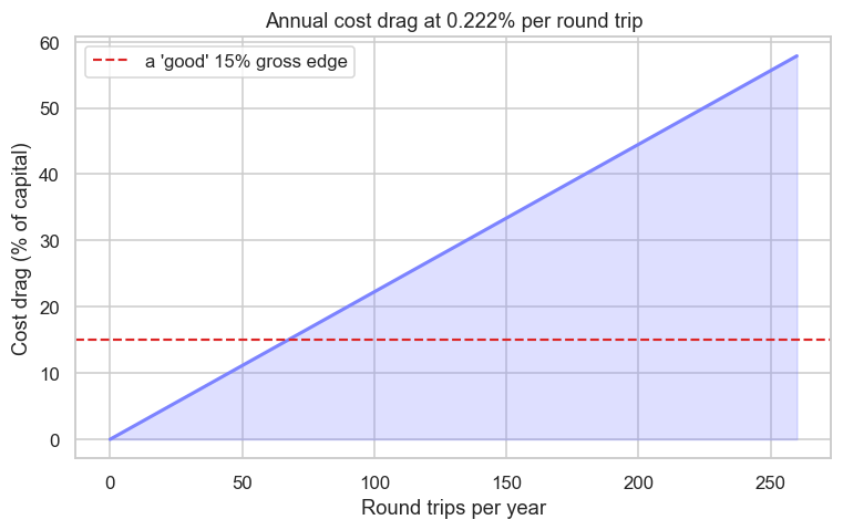
The line is brutal. At just 100 round trips a year - barely two a week - costs alone eat over 22% of your capital. A strategy turning over daily can hand more than half its capital to costs before the market even has an opinion. That red line is a genuinely good 15% gross edge, and the cost curve blows straight through it: trade often enough and your beautiful edge is entirely consumed by friction.

This single chart explains why high-frequency strategies need either a razor-thin cost structure (the domain of HFT and prop desks, Module B) or an edge per trade large enough to clear the hurdle. For everyone else, it's a quiet argument for trading less, and bigger.

The quant's cost rule

It comes down to one equation you must never forget:

net edge = gross edge − costs

Your strategy doesn't keep what it makes; it keeps what's left after friction. So a quant builds the cost model before getting excited about a backtest, and every backtest in this course (and the whole of Module H) runs with realistic costs baked in. An edge that only exists before costs isn't an edge - it's a donation to the exchange and the government.

Try it yourself

• Compare the four segments. Which is cheapest to trade actively, and why are intraday and options friendlier to a high-turnover strategy than delivery?
• Look at the flat ₹20 brokerage beside the STT line on the delivery trade. Roughly how many times larger is STT than brokerage?
• In the drag chart, lower the per-trade cost to a prop-desk-like 0.02% and re-run. How many trades can you now afford before costs eat a 15% edge?

Recap

• "Zero brokerage" is a myth of omission - a delivery round trip still costs ~0.22% of capital (₹1,112 here), and STT dominates the bill (₹1,000 of it).
• Under the ₹20-per-order discount model many Indian brokers follow, brokerage is a rounding error; the stack is brokerage, STT, exchange charges, SEBI fees, stamp duty and GST, varying by segment.
• Costs compound with frequency: ~0.22% per delivery round trip becomes a 22% annual drag at just 100 trades, swamping even a strong gross edge.
• The rule that governs everything: net edge = gross edge − costs - so model cost first, and backtest with it always on.

We've now mapped the market, traced the plumbing, and counted the cost of playing. With the groundwork laid, we descend into the heart of how prices are really made - the limit order book, where every quant edge is ultimately born or lost.