Capstone: A Full Quant Research Project

This is it - the capstone. Everything in this course converges here, into a single end-to-end project: take an idea, build it with full rigor, and judge it honestly. No new theory - just the entire craft applied at once, exactly as a working quant would. And the result, drawn from real Nifty data, delivers the most important lesson of the whole course, the one that separates professionals from dreamers. Let's build a strategy properly, and find out what it's really worth.

The hypothesis

We start, as always, with a falsifiable hypothesis and an economic reason (Chapter 27): trends persist, so being long the index when it's above its 50-day average, and out when below, should earn a decent risk-adjusted return. It's a classic, plausible idea with a real story - trend-following works when markets move in sustained directions. Now we test it the right way.

Building it right

We assemble the whole toolkit:

• A lagged signal (Chapter 32) - the trend decision uses only yesterday's data, so there's no look-ahead.
• Volatility targeting (Chapter 25) - we scale exposure toward a 12% annual volatility, trading smaller when the market is wild.
• Realistic costs (Chapter 4) - every change in position is charged friction, so we judge the strategy net, the way it would actually trade.
• An out-of-sample split (Chapter 27) - we look at the first 60% of history and the held-out last 40% separately.

# CAPSTONE: a complete, HONEST strategy - lagged signal, vol-targeting, costs, out-of-sample.
import os
from datetime import datetime

import numpy as np
from openalgo import api

client = api(
    api_key=os.getenv("OPENALGO_API_KEY", "your_api_key_here"),
    host=os.getenv("OPENALGO_HOST", "http://127.0.0.1:5000"),
)

end = datetime.now().strftime("%Y-%m-%d")
c = client.history(symbol="NIFTY", exchange="NSE_INDEX", interval="D",
                   start_date="2019-01-01", end_date=end)["close"]
r = c.pct_change()

# 1. SIGNAL (hypothesis: trend) - LAGGED so there is no look-ahead (Ch32)
signal = np.sign(c - c.rolling(50).mean()).shift(1)
# 2. VOLATILITY TARGETING - scale exposure toward 12% annual vol (Ch25)
target = 0.12 / np.sqrt(252)
exposure = (target / r.rolling(20).std()).clip(upper=2.0).shift(1)
position = signal * exposure
# 3. COSTS - charge realistic friction on every change in position (Ch4)
strat = position * r - position.diff().abs() * 0.0002


def report(x, label):
    x = x.dropna()
    eq = (1 + x).cumprod()
    sharpe = x.mean() / x.std() * np.sqrt(252)
    cagr = (eq.iloc[-1] ** (252 / len(x)) - 1) * 100
    maxdd = (eq / eq.cummax() - 1).min() * 100
    print(f"{label:16s} Sharpe {sharpe:+.2f}   CAGR {cagr:+5.1f}%   MaxDD {maxdd:5.1f}%")


split = int(len(c) * 0.6)                       # 4. OUT-OF-SAMPLE split (Ch27)
print("Trend + vol-target + costs, NIFTY:")
report(strat[:split], "  in-sample")
report(strat[split:], "  out-of-sample")
report(r[split:], "  buy & hold (OOS)")
print("\nThe out-of-sample line, net of costs, is the only verdict that counts.")

Trend + vol-target + costs, NIFTY:
  in-sample      Sharpe +0.87   CAGR +11.2%   MaxDD -20.1%
  out-of-sample  Sharpe +0.23   CAGR  +2.3%   MaxDD -13.6%
  buy & hold (OOS) Sharpe +0.71   CAGR  +8.9%   MaxDD -15.8%

The out-of-sample line, net of costs, is the only verdict that counts.

The honest verdict

Now read the output slowly, because it's the climax of the entire course. In-sample, the strategy looks respectable - a Sharpe of 0.87. But out-of-sample, net of costs, it managed only 0.23 - and plain buy-and-hold did 0.71. Our clever trend strategy, built with every technique in this book, lost to simply holding the index. The tearsheet makes it unmistakable:

Copy

# The capstone tearsheet: equity curve vs buy-and-hold, with drawdown - the honest picture.
import os
from datetime import datetime
from pathlib import Path

import matplotlib

matplotlib.use("Agg")
import matplotlib.pyplot as plt
import numpy as np
import seaborn as sns
from openalgo import api

client = api(
    api_key=os.getenv("OPENALGO_API_KEY", "your_api_key_here"),
    host=os.getenv("OPENALGO_HOST", "http://127.0.0.1:5000"),
)

end = datetime.now().strftime("%Y-%m-%d")
c = client.history(symbol="NIFTY", exchange="NSE_INDEX", interval="D",
                   start_date="2019-01-01", end_date=end)["close"]
r = c.pct_change()

signal = np.sign(c - c.rolling(50).mean()).shift(1)
exposure = (0.12 / np.sqrt(252) / r.rolling(20).std()).clip(upper=2.0).shift(1)
strat = (signal * exposure * r - (signal * exposure).diff().abs() * 0.0002).fillna(0)

eq_strat = (1 + strat).cumprod()
eq_hold = (1 + r.fillna(0)).cumprod()
dd = (eq_strat / eq_strat.cummax() - 1) * 100
split = int(len(c) * 0.6)

sns.set_theme(style="whitegrid")
fig, (ax1, ax2) = plt.subplots(2, 1, figsize=(8, 6), sharex=True,
                               gridspec_kw={"height_ratios": [3, 1]})
ax1.plot(eq_strat.index, eq_strat, color="#7c83ff", lw=1.6, label="strategy (net of costs)")
ax1.plot(eq_hold.index, eq_hold, color="#888", lw=1.3, ls="--", label="buy & hold")
ax1.axvline(eq_strat.index[split], color="#dc2626", lw=1, ls=":")
ax1.text(eq_strat.index[split], eq_strat.max() * 0.6, " out-of-sample ->", color="#dc2626", fontsize=9)
ax1.set_title("Capstone: trend + vol-target + costs vs buy-and-hold")
ax1.set_ylabel("Growth of 1")
ax1.legend(loc="upper left")
ax2.fill_between(dd.index, dd, 0, color="#dc2626", alpha=0.3)
ax2.set_ylabel("Drawdown %")

out = Path(__file__).with_suffix(".png")
plt.savefig(out, dpi=110, bbox_inches="tight")
print(f"Strategy {eq_strat.iloc[-1]:.2f}x vs buy-hold {eq_hold.iloc[-1]:.2f}x, worst drawdown {dd.min():.0f}%. Saved {out.name}")

Live output

Strategy 1.67x vs buy-hold 2.20x, worst drawdown -20%. Saved 02_capstone_tearsheet.png

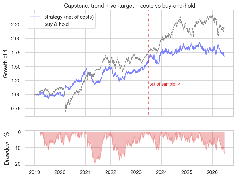
The strategy curve (1.67x) trails buy-and-hold (2.20x), with a 20% drawdown for its trouble. By the naive standard, the project "failed".

The most important lesson in the course

But it did not fail - it succeeded, completely. The goal of research was never to make this idea work; it was to find out, honestly and cheaply, before risking a rupee, whether it works. And the process did exactly that: it told us, clearly, that a simple trend filter doesn't beat buy-and-hold on the Nifty after costs. We learned that for the price of an afternoon's coding instead of a year of real losses. That is what the entire course has been building toward.

What a real edge requires

So where do the durable edges live? Not, usually, in a lone directional filter on a liquid index - that's the most efficient, most competed corner of the market (Chapter 14). They live in the places this course pointed to: market-neutral relationships that don't even try to beat the index (stat-arb, Chapter 28); diversified multi-factor books held over long horizons (Chapter 24); structural and event-driven edges from forced flows (Chapter 30); volatility harvested with discipline (Chapter 22); and combinations of several uncorrelated edges sized by risk (Chapter 25). A real strategy is rarely one clever signal - it's a portfolio of honest, modest, uncorrelated edges, each one having survived the gauntlet we just ran.

The full pipeline

This capstone is the whole course in one diagram - the pipeline every idea must pass through:

Where to go from here

You finish this course able to do something rare: take a trading idea and determine, rigorously and honestly, whether it holds up - and build it on real Indian market data with the OpenAlgo SDK. That skill is the foundation of everything. From here: research more ideas (most will fail the gauntlet - that's normal), combine the survivors into a diversified book, sandbox-trade relentlessly in analyzer mode before going live, size with humility, and never stop being skeptical of your own backtests. The market will always try to fool you; your job, now well-trained, is to refuse.

Recap

• The capstone runs an idea through the entire pipeline: hypothesis, clean data, lagged signal, vol-targeted sizing, realistic costs, out-of-sample test.
• The honest verdict: a plausible trend strategy looked good in-sample (0.87) but lost to buy-and-hold out-of-sample (0.23 vs 0.71) after costs.
• That's a success, not a failure - the process correctly killed a weak idea cheaply, before any real money was at risk.
• Durable edges live in market-neutral, multi-factor, event-driven and volatility strategies, combined as a diversified book - rarely in a lone directional filter on a liquid index.
• The defining quant skill isn't prediction; it's the rigor and honesty to tell a real edge from a flattering backtest - and to trade only the real ones.

You've reached the end. You now have the full toolkit of a quant - market structure, the mathematics of markets, derivatives, portfolio risk, the strategy families, and the discipline that ties them together - all grounded in Indian markets and built on real data. Go research, test honestly, trade in analyze mode first, and build something real. Welcome to quant.