Stationarity & the Random Walk

We've armed ourselves against fake edges. Now the harder question: is there any real edge to find at all? Can a price even be predicted? The uncomfortable, foundational answer is that a price behaves astonishingly like a random walk - a path with no memory, no anchor, and no obligation to go anywhere. Understanding exactly how unpredictable prices are - and the precise, narrow ways they aren't - is what tells a quant where to hunt and where to give up. This chapter closes the mathematics module with the deepest idea of all.

The random walk

Imagine a drunk leaving a bar, each step a random stagger in some direction. Where will they be in an hour? You genuinely cannot say - the path wanders, and crucially, each step is independent of the last. A random walk is exactly this: tomorrow's value is today's value plus an unpredictable shock. Prices look uncannily like this, which is the whole problem. If price is a random walk, then the past tells you nothing about the next step's direction - studying the chart harder buys you nothing.

Stationary versus non-stationary

The technical word for "has no anchor" is non-stationary: a series whose mean and variance drift over time, wandering off with no level to return to. Its opposite is stationary: a series pulled back toward a stable mean, with consistent variance - something you can actually model, because its statistical character doesn't change.

This is why, all through the course, we work with returns and not raw prices. Returns are stationary - they bounce around a stable, tiny mean - so they have a consistent character you can study and model. Prices are non-stationary - they wander - so any model fitted to price levels quietly breaks the moment the price wanders somewhere new.

The ADF test

You don't have to eyeball it - there's a formal test. The Augmented Dickey-Fuller (ADF) test takes a series and asks, "is this a random walk?" Its null hypothesis is non-stationary; a small p-value lets you reject that and call the series stationary. Let's run it on Nifty's price and its returns:

# Are prices predictable? The ADF test asks: is this just a random walk?
import os
from datetime import datetime

from openalgo import api
from statsmodels.tsa.stattools import adfuller

client = api(
    api_key=os.getenv("OPENALGO_API_KEY", "your_api_key_here"),
    host=os.getenv("OPENALGO_HOST", "http://127.0.0.1:5000"),
)

end = datetime.now().strftime("%Y-%m-%d")
p = client.history(symbol="NIFTY", exchange="NSE_INDEX", interval="D",
                   start_date="2021-01-01", end_date=end)["close"]
r = p.pct_change().dropna()

# ADF null hypothesis: the series is NON-stationary (a random walk with a unit root).
# A small p-value (< 0.05) lets us reject that and call it stationary.
adf_price = adfuller(p)
adf_ret = adfuller(r)


def verdict(pval):
    return "STATIONARY (mean-reverting)" if pval < 0.05 else "NON-stationary (random walk)"


print("ADF test  (null = random walk):")
print(f"  NIFTY price   : stat {adf_price[0]:6.2f}   p-value {adf_price[1]:.3f}   -> {verdict(adf_price[1])}")
print(f"  NIFTY returns : stat {adf_ret[0]:6.2f}   p-value {adf_ret[1]:.3f}   -> {verdict(adf_ret[1])}")
print("\nPrice wanders with no anchor; returns are stationary - which is why quants model RETURNS, not price.")

ADF test  (null = random walk):
  NIFTY price   : stat  -1.49   p-value 0.538   -> NON-stationary (random walk)
  NIFTY returns : stat -18.30   p-value 0.000   -> STATIONARY (mean-reverting)

Price wanders with no anchor; returns are stationary - which is why quants model RETURNS, not price.

The verdict is emphatic. Nifty's price has a p-value of 0.54 - nowhere near significant, so we cannot reject the random walk; the price genuinely behaves like a drunk's stagger. Its returns, though, have a p-value of essentially zero - decisively stationary. This single pair of numbers justifies the entire modelling philosophy of quant finance: don't model the wandering price, model the well-behaved returns.

See it

The contrast is just as clear to the eye:

Copy

# See stationarity: price wanders with no anchor, returns snap back to a mean.
import os
from datetime import datetime
from pathlib import Path

import matplotlib

matplotlib.use("Agg")
import matplotlib.pyplot as plt
import seaborn as sns
from openalgo import api
from statsmodels.tsa.stattools import adfuller

client = api(
    api_key=os.getenv("OPENALGO_API_KEY", "your_api_key_here"),
    host=os.getenv("OPENALGO_HOST", "http://127.0.0.1:5000"),
)

end = datetime.now().strftime("%Y-%m-%d")
df = client.history(symbol="NIFTY", exchange="NSE_INDEX", interval="D",
                    start_date="2021-01-01", end_date=end)
p = df["close"]
r = p.pct_change().dropna() * 100

sns.set_theme(style="whitegrid")
fig, ax = plt.subplots(2, 1, figsize=(8, 6), sharex=True)

ax[0].plot(p.index, p, color="#7c83ff", lw=1.3)
ax[0].set_title(f"NIFTY price - NON-stationary (ADF p = {adfuller(p)[1]:.2f}): wanders off")
ax[0].set_ylabel("Price")

ax[1].plot(r.index, r, color="#16a34a", lw=0.7)
ax[1].axhline(r.mean(), color="#dc2626", lw=1.4, label=f"mean {r.mean():.2f}%")
ax[1].set_title(f"NIFTY daily returns - STATIONARY (ADF p = {adfuller(r)[1]:.3f}): pulled to a mean")
ax[1].set_ylabel("Return (%)")
ax[1].legend()

fig.tight_layout()
out = Path(__file__).with_suffix(".png")
plt.savefig(out, dpi=110, bbox_inches="tight")
print(f"Price ADF p={adfuller(p)[1]:.2f} (random walk), returns ADF p={adfuller(r)[1]:.3f} (stationary). Saved {out.name}")

Live output

Price ADF p=0.54 (random walk), returns ADF p=0.000 (stationary). Saved 02_stationarity.png

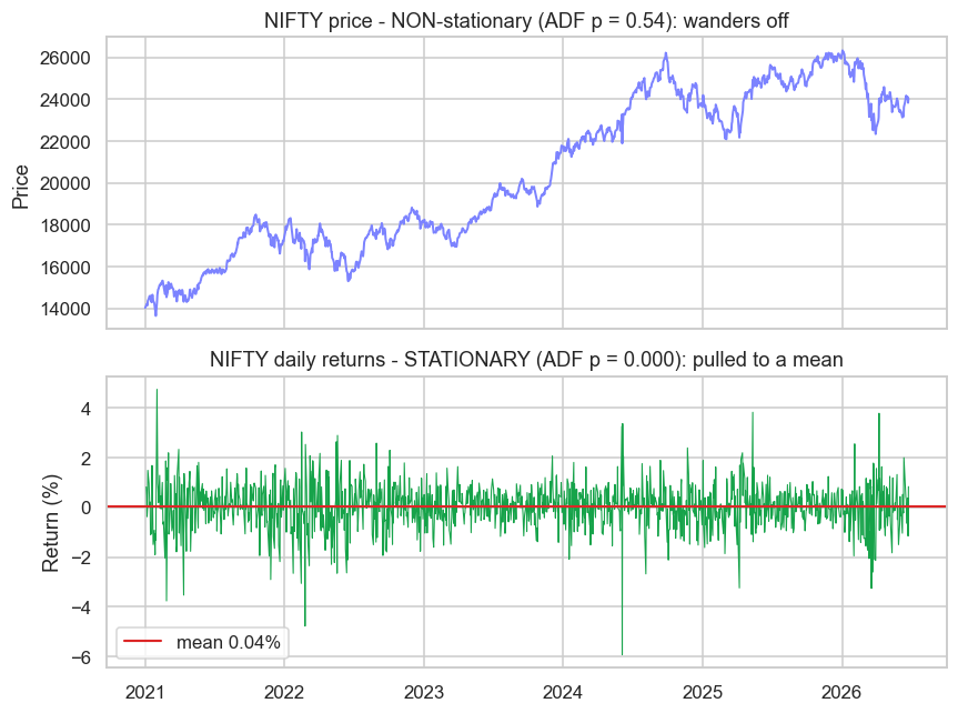
The top panel wanders off across years with no level it's drawn to; the bottom panel hugs a flat red mean line, every excursion yanked back. One you can model; one you can't.

The efficient market hypothesis

If prices are a random walk, then all the information that could be known is already baked into the price, and the next move is driven only by new information - which is, by definition, unpredictable. That's the efficient market hypothesis (EMH), and it comes in grades: the weak form says past prices can't predict the future (technical analysis is futile); the semi-strong form says public information is already priced in; the strong form says even private information is. Taken literally, the EMH says no edge can exist. The ADF result above is the EMH showing its teeth.

Where the EMH cracks

But the market is mostly efficient, not perfectly so - and a quant lives in the gap. The cracks are real and documented:

• Anomalies that persist - momentum, value, low-volatility - earn returns the strict EMH says shouldn't exist (Module F).
• Fat tails and volatility clustering (Chapter 11) violate the neat random-walk model; risk, at least, is predictable.
• Behavioural biases - herding, overreaction, anchoring - create patterns, because the market is made of humans, not perfectly rational machines.
• Structural quirks - forced flows from index rebalancing, expiry effects, segment frictions - leave footprints (Module G).

Try it yourself

• Run the ADF test on a single stock's price and returns. Do you get the same pattern - price non-stationary, returns stationary?
• Test the spread between two related stocks (say HDFCBANK − ICICIBANK). Is the spread stationary even though each price isn't? (That hint is the heart of Chapter 17.)
• Simulate a pure random walk with numpy.cumsum of random steps and run ADF on it. Confirm it tests as non-stationary, just like a real price.

Recap

• A random walk has no memory and no anchor - tomorrow is today plus an unpredictable shock - and prices behave remarkably like one.
• Non-stationary series (prices) wander with drifting mean and variance; stationary series (returns) revert to a stable mean and can be modelled.
• The ADF test formalises it: Nifty's price tests as a random walk (p = 0.54), its returns as decisively stationary (p ≈ 0) - which is why quants model returns.
• The efficient market hypothesis says a random-walk price has already priced in all information, so the next move is unpredictable.
• The market is mostly but not perfectly efficient - anomalies, fat tails, behavioural biases and structural quirks are the real cracks where genuine edges live.

That completes Module C - the mathematics of returns, probability, honest inference, and the random walk. We now have the tools to model what little structure markets do have. Module D puts them to work: time-series models, volatility that clusters, and the mean-reversion that powers an entire class of strategies.