Probability & Monte Carlo

Here's a fact that ruins more traders than any bad strategy: a genuinely winning system can lose money for a year, and a losing system can win for months. The reason is luck - the randomness that sits on top of every edge. A quant's superpower is the ability to separate the two: to ask, coldly, "is this result skill, or did the dice just fall my way?" The language for that question is probability, and the tool that makes it practical is Monte Carlo simulation. Let's learn both, gently.

Expectation: the average outcome

A single trade is a random variable - you don't know the result in advance, only the possible outcomes and their chances. The expectation (or expected value) is the probability-weighted average of those outcomes: what you'd get per trade if you ran it thousands of times. Let's measure it for the simplest possible rule - just holding Nifty for a day:

# Expectation is the long-run average outcome. Let's measure a simple rule's expectancy.
import os
from datetime import datetime, timedelta

from openalgo import api

client = api(
    api_key=os.getenv("OPENALGO_API_KEY", "your_api_key_here"),
    host=os.getenv("OPENALGO_HOST", "http://127.0.0.1:5000"),
)

end = datetime.now().strftime("%Y-%m-%d")
start = (datetime.now() - timedelta(days=730)).strftime("%Y-%m-%d")
r = client.history(symbol="NIFTY", exchange="NSE_INDEX", interval="D",
                   start_date=start, end_date=end)["close"].pct_change().dropna() * 100

wins, losses = r[r > 0], r[r < 0]
win_rate = len(wins) / len(r)
avg_win, avg_loss = wins.mean(), losses.mean()
expectancy = win_rate * avg_win + (1 - win_rate) * avg_loss

print(f"Win rate    : {win_rate * 100:.1f}%")
print(f"Average win : +{avg_win:.2f}%")
print(f"Average loss: {avg_loss:.2f}%")
print(f"\nExpectancy  : {expectancy:+.3f}% per day  (probability-weighted average outcome)")
print(f"Actual mean : {r.mean():+.3f}% per day  (matches - expectancy IS the expected value)")

Win rate    : 50.8%
Average win : +0.61%
Average loss: -0.62%

Expectancy  : +0.008% per day  (probability-weighted average outcome)
Actual mean : +0.008% per day  (matches - expectancy IS the expected value)

The expectancy (+0.008% per day) is computed two ways - the weighted average of wins and losses, and the plain mean of every day - and they match exactly, because that's what expectation is. This tiny positive number is the entire edge of buy-and-hold: small per day, but relentless. Every strategy lives or dies by whether its expectancy is positive after costs.

Variance: the spread around the average

Expectation tells you the centre; it says nothing about the ride. Variance (and its square root, standard deviation) measures how far outcomes scatter around the expectation. Two strategies can share an expectancy of +0.5% per trade, but one delivers it smoothly and the other through stomach-churning swings. The smooth one is worth far more - same reward, less risk - which is why a quant always reports expectation and variance together. Never one without the other.

The law of large numbers

Here's the catch that traps beginners. Expectation is a long-run average - it only reveals itself over many trials. The law of large numbers says the average of your results converges to the true expectation as the number of trades grows - but over a small sample, luck dominates completely. Twenty trades tell you almost nothing; a thousand start to tell the truth.

Monte Carlo: roll the dice thousands of times

So how do you see the role of luck before it costs you real money? You simulate it. Monte Carlo simulation takes your real outcomes and reshuffles them into thousands of alternate histories, revealing the full range of where the same edge could land you:

Copy

# Monte Carlo: resample real Nifty days to see the RANGE of luck over a year.
import os
from datetime import datetime
from pathlib import Path

import matplotlib

matplotlib.use("Agg")
import matplotlib.pyplot as plt
import numpy as np
import seaborn as sns
from openalgo import api

client = api(
    api_key=os.getenv("OPENALGO_API_KEY", "your_api_key_here"),
    host=os.getenv("OPENALGO_HOST", "http://127.0.0.1:5000"),
)

end = datetime.now().strftime("%Y-%m-%d")
df = client.history(symbol="NIFTY", exchange="NSE_INDEX", interval="D",
                    start_date="2021-01-01", end_date=end)
log_r = np.log(df["close"] / df["close"].shift(1)).dropna().values

rng = np.random.default_rng(7)            # seeded, so the run is reproducible
N_SIMS, DAYS = 500, 252
sims = np.array([100 * np.exp(np.cumsum(rng.choice(log_r, size=DAYS, replace=True)))
                 for _ in range(N_SIMS)])

sns.set_theme(style="whitegrid")
fig, ax = plt.subplots(figsize=(8, 4.5))
for path in sims[:200]:
    ax.plot(path, color="#7c83ff", alpha=0.05)
ax.plot(np.percentile(sims, 50, axis=0), color="#16a34a", lw=2, label="median outcome")
ax.plot(np.percentile(sims, 5, axis=0), color="#dc2626", lw=1.5, ls="--", label="5th / 95th percentile")
ax.plot(np.percentile(sims, 95, axis=0), color="#dc2626", lw=1.5, ls="--")
ax.set_title("500 simulated years of Nifty - the same edge, very different luck")
ax.set_xlabel("Trading day")
ax.set_ylabel("Growth of 100")
ax.legend()

out = Path(__file__).with_suffix(".png")
plt.savefig(out, dpi=110, bbox_inches="tight")
finals = sims[:, -1]
print(f"After 1 year - median {np.median(finals):.0f}, "
      f"unlucky 5th {np.percentile(finals, 5):.0f}, lucky 95th {np.percentile(finals, 95):.0f}. Saved {out.name}")

Live output

After 1 year - median 111, unlucky 5th 87, lucky 95th 138. Saved 02_monte_carlo.png

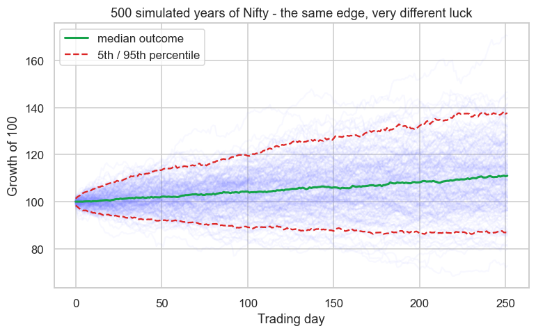
Look at the fan. Every one of those 500 faint paths has the exact same edge - they're all built by resampling the same real Nifty days - yet after one year they scatter from a miserable 87 to a delightful 138. The median lands near 111, but the 5th-to-95th-percentile spread is the footprint of luck: the range of outcomes you could get through no skill or fault of your own. A trader who happened to ride the top path would feel like a genius; one on the bottom path, a failure. Same edge, different dice.

Why quants simulate

When a payoff is simple, a formula gives you the expectation directly. But real strategies are path-dependent - drawdowns, trailing stops, risk-of-ruin, position sizing that changes with your equity - and no clean formula exists. Monte Carlo is how a quant answers the questions that matter most:

• What's the worst drawdown I should expect even if my edge is real?
• What's the chance I blow up before the edge plays out?
• How wide is the range of outcomes - is this a smooth edge or a lottery?

It replaces "what's the average?" with the far more useful "what's the whole distribution of what could happen?" - and that shift, from a single number to a range, is the heart of thinking probabilistically.

Try it yourself

• Re-run the Monte Carlo with DAYS = 1260 (five years). Does the gap between the lucky and unlucky paths widen or narrow over a longer horizon?
• Compute the expectancy of a down-day rule (short Nifty each day). Is it negative, as you'd expect from the index's slight upward drift?
• Add a column to the simulation for the worst drawdown of each path. What's the median worst-drawdown a buy-and-hold investor should brace for?

Recap

• A trade is a random variable; its expectation is the probability-weighted average outcome - the edge per bet, which must be positive after costs.
• Variance measures the spread around that average - always report expectation and variance, because the smoothness of the ride is worth real money.
• The law of large numbers means an edge only shows over many trades; small samples are dominated by luck and prove nothing.
• Monte Carlo reshuffles real outcomes into thousands of alternate histories, revealing the full range of luck - the same edge can land anywhere between unlucky and lucky.
• Quants simulate because real strategies are path-dependent, and the useful question isn't "what's the average?" but "what's the whole distribution of what could happen?"

We've learned to reason about a single random outcome. Next we confront the trap that catches even smart quants: when you test hundreds of ideas, randomness guarantees some will look brilliant by pure chance - the multiple-testing problem, and how to not fool yourself.