Module F · Portfolio Construction & Risk - Chapter 26

Tail Risk: VaR, CVaR & Stress

Your worst normal day, and the days that break the model - VaR, expected shortfall and stress testing.

NSEINDEX

What you'll learn

·Value at Risk (VaR)
·Historical vs parametric VaR
·Expected shortfall (CVaR)
·Stress testing
·Drawdown control
·Indian shock case studies

Everything so far has sized risk for the normal world. But accounts don't die in the normal world - they die in the tail, on the one day in years when the market does something the bell curve swore was impossible. Chapter 11 proved those days come far more often than the model admits; this chapter is about surviving them. Measuring tail risk, respecting how badly your measures fail, and stress-testing for the shock that hasn't happened yet - this is the discipline that separates a quant who lasts decades from one who has a great two years and then vanishes.

Value at Risk

The industry's standard tail metric is Value at Risk (VaR): the loss you won't exceed with some confidence, over some horizon. A 95% one-day VaR of −1.5% means "on 19 days out of 20, you won't lose more than 1.5%." Let's compute it on Nifty, across a window that includes the COVID crash:

EX 1Value at Risk and beyondINDEXch26/01_var.py

# Value at Risk: the loss to expect on a bad day - and the deeper truth beyond it.
import os
from datetime import datetime

import numpy as np
from openalgo import api
from scipy import stats

client = api(
    api_key=os.getenv("OPENALGO_API_KEY", "your_api_key_here"),
    host=os.getenv("OPENALGO_HOST", "http://127.0.0.1:5000"),
)

end = datetime.now().strftime("%Y-%m-%d")
r = client.history(symbol="NIFTY", exchange="NSE_INDEX", interval="D",
                   start_date="2019-01-01", end_date=end)["close"].pct_change().dropna() * 100

hist_var95 = np.percentile(r, 5)                              # 95% VaR from real history
hist_var99 = np.percentile(r, 1)                             # 99% VaR
param_var99 = stats.norm.ppf(0.01, r.mean(), r.std())        # 99% VaR assuming normal
cvar95 = r[r <= hist_var95].mean()                           # expected shortfall

print(f"95% 1-day VaR (historical) : {hist_var95:.2f}%   - lose at least this ~1 day in 20")
print(f"99% 1-day VaR (historical) : {hist_var99:.2f}%   - ~1 day in 100")
print(f"99% 1-day VaR (normal model): {param_var99:.2f}%   - the bell curve UNDERSTATES the tail")
print(f"\n95% CVaR / expected shortfall: {cvar95:.2f}%   - the AVERAGE loss on the worst 5% of days")
print(f"Worst actual day             : {r.min():.2f}%   - far beyond any VaR (COVID, Mar 2020)")
print("\nVaR is the line; CVaR is how bad it gets beyond it. Fat tails make 'beyond' ugly.")

Live output

95% 1-day VaR (historical) : -1.51%   - lose at least this ~1 day in 20
99% 1-day VaR (historical) : -2.98%   - ~1 day in 100
99% 1-day VaR (normal model): -2.52%   - the bell curve UNDERSTATES the tail

95% CVaR / expected shortfall: -2.58%   - the AVERAGE loss on the worst 5% of days
Worst actual day             : -12.98%   - far beyond any VaR (COVID, Mar 2020)

VaR is the line; CVaR is how bad it gets beyond it. Fat tails make 'beyond' ugly.

The historical 95% VaR is −1.5%, the 99% VaR −3.0%. VaR is useful shorthand - a single number for "a normal bad day." But read the rest of that output, because it exposes two flaws that have cost real institutions their existence.

VaR's two fatal flaws

First, VaR is silent about how bad it gets beyond the line. It says you'll lose at least 3% on the worst 1% of days - but says nothing about whether that's 3% or 13%. And look at the worst actual day: −12.98% (COVID, March 2020), more than four times the 99% VaR. VaR drew a line and the market leapt clean over it.

Second, the normal-model VaR understates the danger. The parametric (bell-curve) 99% VaR came out at −2.5%, milder than the −3.0% the real, fat-tailed history delivered. Assume normality - as countless risk systems did before 2008 - and you systematically under-reserve for exactly the events that destroy you.

Expected shortfall (CVaR)

The fix for the first flaw is expected shortfall, or CVaR: instead of the threshold, it measures the average loss across the entire tail beyond VaR. It answers "when things go bad, how bad on average?"

VaR marks the line; CVaR is the average of everything beyond it

CVaR came out at −2.6% - worse than the 95% VaR, because it includes those brutal far-tail days the threshold ignored. CVaR is the metric serious risk managers (and modern regulation) increasingly prefer, precisely because it cannot hide the depth of the tail behind a single comfortable number.

The drawdown that matters

VaR and CVaR are about a single day. What you actually live through is the drawdown - the cumulative fall from a previous peak, the slow underwater agony that tests your nerve and your investors' patience:

The underwater drawdown chart chart — EX 2The underwater drawdown chartINDEXch26/02_drawdown.py

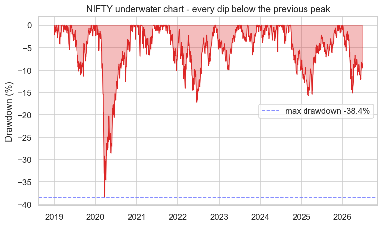
The underwater chart is honest in a way daily VaR never is. Nifty's worst drawdown since 2019 was −38% - more than a third of capital gone, over weeks, with no certainty at the bottom that it would ever recover. That is the experience a risk number must prepare you for: not one bad day, but a long, deep, terrifying decline. Controlling maximum drawdown - through sizing, stops and hedges - is often the real objective, because it's the drawdown, not the daily VaR, that makes people abandon a sound strategy at the worst possible moment.

Stress testing

History only contains the shocks that happened. Stress testing asks about the ones that could: what does my book lose if Nifty gaps down 10% overnight, if volatility triples, if a currency crisis hits, if liquidity vanishes? Rather than trusting a statistical model, you impose specific, brutal scenarios and read the damage directly. A quant who has stress-tested for a −15% gap is not surprised when one arrives - and isn't over-sized into it.

Indian shocks are real and recurring

India offers no shortage of tail events to learn from: the COVID crash of March 2020 (the −13% day, the −38% drawdown), demonetisation in 2016, the 2024 election-result day that swung violently intraday, recurring global contagions. These aren't ancient history or foreign curiosities - they're a recurring feature of the market you trade, and any risk framework that treats them as once-in-a-millennium flukes is lying to you.

Key idea

Size for the tail, not the average. VaR is a useful summary but it hides the depth of the tail and, under a normal assumption, understates it - so lean on CVaR, watch drawdown, and stress-test for shocks history hasn't shown you yet. The market's worst day is always still ahead of you; the only question is whether you're sized to survive it.

Try it yourself

Compute VaR and CVaR for a single high-beta stock. How much fatter is its tail than the index's?
Stress-test a leveraged position: if Nifty gapped −10% overnight, what would a 2x-levered book lose, and would it survive?
Measure the recovery time of the COVID drawdown - how many months from the bottom back to a new high? That duration is the patience your risk model must assume.

Recap

Value at Risk (VaR) is the loss you won't exceed at a given confidence - a useful summary of a normal bad day (95% Nifty VaR ≈ −1.5%).
VaR has two fatal flaws: it's silent about the depth beyond the line (the −13% COVID day dwarfed the −3% 99% VaR), and the normal model understates the fat-tailed truth.
Expected shortfall (CVaR) fixes the first flaw by averaging the entire tail beyond VaR - the metric serious risk managers prefer.
Drawdown - the underwater fall from a peak - is what you actually live through; Nifty's −38% COVID drawdown is the kind of pain risk control must prepare for.
Stress test for shocks history hasn't shown, learn from India's real tail events, and always size for the tail - the worst day is still ahead.

That completes Module F - we can now build a portfolio, size it, and guard its tail. Everything so far has been foundations. Module G is where it pays off: the actual process of finding an edge, and the families of strategies - stat-arb, momentum, event-driven, market-making - that turn all this theory into alpha.