Factor Models & Equity Risk

Why does a stock go up? Most of the answer isn't company-specific at all - it's a handful of deep, market-wide forces that drive whole groups of stocks together. These forces are called factors, and they're the closest thing quant equity investing has to a periodic table: a small set of return drivers that explain most of what happens, and that you can deliberately tilt toward. Understanding factors turns stock-picking from a guessing game into a systematic exposure decision. But - as this chapter's data will show with brutal honesty - factors are also where over-eager quants fool themselves most.

The first factor: the market

The biggest force on any stock is simply the market itself. When Nifty moves, almost everything moves with it - just by different amounts. That sensitivity is beta, the heart of the CAPM: a beta of 1 means the stock moves one-for-one with the market, above 1 amplifies it, below 1 dampens it. Let's measure a few:

# CAPM beta: how much a stock amplifies (or dampens) the market's moves.
import os
from datetime import datetime, timedelta

import numpy as np
import pandas as pd
from openalgo import api

client = api(
    api_key=os.getenv("OPENALGO_API_KEY", "your_api_key_here"),
    host=os.getenv("OPENALGO_HOST", "http://127.0.0.1:5000"),
)

end = datetime.now().strftime("%Y-%m-%d")
start = (datetime.now() - timedelta(days=730)).strftime("%Y-%m-%d")

mkt = client.history(symbol="NIFTY", exchange="NSE_INDEX", interval="D",
                     start_date=start, end_date=end)["close"].pct_change()

print(f"{'STOCK':12s}{'BETA':>7s}   reads as")
for sym in ["TATASTEEL", "ADANIENT", "HDFCBANK", "ITC", "HINDUNILVR"]:
    s = client.history(symbol=sym, exchange="NSE", interval="D",
                       start_date=start, end_date=end)["close"].pct_change()
    df = pd.concat([mkt, s], axis=1).dropna()
    beta = np.cov(df.iloc[:, 1], df.iloc[:, 0])[0, 1] / np.var(df.iloc[:, 0])
    tag = "high beta - amplifies the market" if beta > 1 else "low beta - defensive"
    print(f"{sym:12s}{beta:>7.2f}   {tag}")

print("\nBeta is your exposure to the MARKET factor - the first and biggest driver of a stock's return.")

STOCK          BETA   reads as
TATASTEEL      1.27   high beta - amplifies the market
ADANIENT       1.62   high beta - amplifies the market
HDFCBANK       1.05   high beta - amplifies the market
ITC            0.61   low beta - defensive
HINDUNILVR     0.55   low beta - defensive

Beta is your exposure to the MARKET factor - the first and biggest driver of a stock's return.

The spread is exactly what your intuition expects. Adani Enterprises (1.62) and Tata Steel (1.27) are high-beta - they amplify every market swing, soaring in rallies and cratering in falls. The FMCG defensives, ITC (0.61) and Hindustan Unilever (0.55), are low-beta - they barely flinch when the market lurches. Beta is your first and largest exposure: before any clever signal, a chunk of your return is just the market, scaled.

Beyond the market: the factor zoo

The market is factor number one, but it's not the only one. Decades of research - starting with Fama and French - found a handful of other forces that systematically drive returns:

In plain words: value (cheap stocks beat expensive ones over time), momentum (recent winners tend to keep winning), quality (profitable, stable companies outperform), low volatility (calmer stocks deliver better risk-adjusted returns - a genuine anomaly), and size (small-caps carry a premium for their extra risk). Tilt a portfolio toward these and, over the long run and across many names, you're harvesting documented sources of return.

Testing momentum - honestly

But "over the long run" hides a trap, and this chapter's second example walks straight into it. Let's test momentum on Indian stocks: rank them by last year's return, then see if the winners kept winning this year:

Copy

# A momentum factor: do last year's winners keep winning? Rank, then check next year.
import os
from datetime import datetime, timedelta
from pathlib import Path

import matplotlib

matplotlib.use("Agg")
import matplotlib.pyplot as plt
import pandas as pd
import seaborn as sns
from openalgo import api

client = api(
    api_key=os.getenv("OPENALGO_API_KEY", "your_api_key_here"),
    host=os.getenv("OPENALGO_HOST", "http://127.0.0.1:5000"),
)

end = datetime.now().strftime("%Y-%m-%d")
start = (datetime.now() - timedelta(days=730)).strftime("%Y-%m-%d")
universe = ["RELIANCE", "INFY", "HDFCBANK", "ITC", "TATASTEEL", "ADANIENT", "SBIN",
            "BHARTIARTL", "MARUTI", "SUNPHARMA", "TITAN", "HINDALCO"]

rows = []
for sym in universe:
    c = client.history(symbol=sym, exchange="NSE", interval="D",
                       start_date=start, end_date=end)["close"]
    mid = len(c) // 2
    rows.append({"stock": sym,
                 "formation": c.iloc[mid] / c.iloc[0] - 1,      # year 1 return (the signal)
                 "holding": c.iloc[-1] / c.iloc[mid] - 1})       # year 2 return (the test)

df = pd.DataFrame(rows).sort_values("formation")
half = len(df) // 2
low, high = df.head(half)["holding"].mean(), df.tail(half)["holding"].mean()

print(f"Low-momentum group, next-year return : {low * 100:+.1f}%")
print(f"High-momentum group, next-year return: {high * 100:+.1f}%")
print(f"Momentum long-short spread           : {(high - low) * 100:+.1f}%")

sns.set_theme(style="whitegrid")
fig, ax = plt.subplots(figsize=(8, 4.5))
sns.regplot(data=df, x="formation", y="holding", ax=ax,
            scatter_kws={"s": 50, "color": "#7c83ff"}, line_kws={"color": "#dc2626"})
ax.set_title("Momentum: last year's return vs next year's (positive slope = momentum works)")
ax.set_xlabel("Formation: year-1 return")
ax.set_ylabel("Holding: year-2 return")
out = Path(__file__).with_suffix(".png")
plt.savefig(out, dpi=110, bbox_inches="tight")
print(f"Saved {out.name}")

Live output

Low-momentum group, next-year return : +24.2%
High-momentum group, next-year return: -11.3%
Momentum long-short spread           : -35.4%
Saved 02_momentum_factor.png

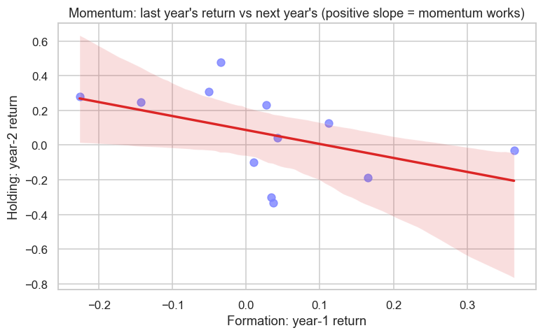
Look at the result - and don't flinch from it. In this window momentum reversed: last year's losers returned +24% while last year's winners fell 11%, a spread of −35%. The regression line slopes the wrong way. Momentum, a factor documented across decades and dozens of markets, completely failed over this particular two-year Indian window. That's not a bug in the code; it's the honest truth about factors.

The factor zoo and its dangers

If that reversal felt uncomfortable, here's the bigger warning. Researchers have published hundreds of supposed factors - the "factor zoo" - and most of them are exactly the multiple-testing mirage of Chapter 13: patterns data-mined from history that evaporate out-of-sample. Only a handful (value, momentum, quality, low-vol, size) have survived decades of scrutiny across many countries, and even those, as we just saw, go through brutal dry spells. Treat any exotic new "factor" with deep suspicion; demand an economic reason it should exist, and out-of-sample proof that it does.

Building India factors

The craft, then, is to build robust factor exposures on the NSE universe: compute each factor cleanly (value from valuation ratios, momentum from trailing returns, low-vol from volatility), combine several of them into a multi-factor score so no single one can sink you, and rebalance patiently. A diversified multi-factor tilt, held for years across a broad universe, is one of the most defensible systematic equity strategies there is - precisely because it doesn't rely on any one factor working in any one year.

Try it yourself

• Re-run the momentum test on a different two-year window. Does momentum work in some periods and reverse in others? (It will - that's the regime-dependence.)
• Build a simple low-volatility factor: rank your universe by trailing volatility and compare the calm half's return to the wild half's. Does the low-vol anomaly show up?
• Combine two factors - rank by momentum and low-vol, average the ranks. Is the combined signal steadier than either alone?

Recap

• Most of a stock's return comes from a few market-wide factors, not company specifics.
• The first and biggest is the market (beta) - high-beta stocks amplify swings (Adani 1.62), low-beta defensives dampen them (HUL 0.55).
• The surviving factors are value, momentum, quality, low-volatility and size - documented, economically-grounded return drivers you can tilt toward.
• Factors are long-run tendencies, not laws: momentum reversed (−35%) over this Indian window - they fail over short horizons and in the wrong regime.
• Beware the factor zoo - most published factors are data-mined noise; build diversified, multi-factor tilts over long horizons on broad universes.

We know what to hold and what drives it. The next question is how much of each - capital allocation and position sizing, where Kelly, risk parity and volatility targeting decide the bet size that keeps you in the game.