Liquidity, Spread & Market Impact

There are two costs to every trade. The first you've already met: the spread, the gap you pay to cross the book. The second is sneakier and, for anyone trading size, far larger - the price you push against yourself simply by trading. Buy enough and you drive the price up before you're done; sell enough and you drive it down. This is liquidity, and putting a number on it is one of the most practical skills a quant has. A strategy that ignores liquidity is a strategy that works on paper and bleeds in the real world.

The three faces of liquidity

Liquidity isn't one thing - it's three, and a good trader watches all of them:

• Spread - the immediate cost of crossing the book (Chapter 5). The tightest, most visible measure.
• Depth - how much you can trade before you start moving the price. A penny spread is useless if only 2 lots sit at it.
• Resilience - how quickly the book refills after you eat into it. A resilient market absorbs your order and snaps back; a fragile one stays dented.

A truly liquid instrument has all three: tight spread, deep book, fast recovery. Most of the market has none of them, which is exactly why thin names are dangerous.

Your order moves the price

Here's the mechanism that surprises every beginner. Say you want to buy 30 lots and the best ask is 6822. You don't get 30 at 6822 - there are only 11 there. So you climb:

Your 30 lots fill across several price levels, each worse than the last, so your average price is meaningfully above the best ask. That gap - between the price you'd have liked and the price you actually got - is market impact (or slippage). It grows with your size and shrinks with the book's depth, and on a thin name it can dwarf brokerage, STT and spread combined.

Kyle's lambda, in one idea

Academics gave this a name: Kyle's lambda (λ). Strip away the maths and it's simply how much the price moves per unit of order flow - the slope of impact against size. A liquid stock has a tiny lambda (trade a lot, barely nudge it); a thin stock has a large lambda (trade a little, shove it). You don't need the equation to use the idea: every market has a price for size, and lambda is that price.

Amihud: liquidity you can measure

Lambda is hard to measure directly, but a brilliant shortcut - the Amihud illiquidity measure - gets you 90% of the way with data you already have. The idea in words: on average, how far does the price move for each rupee traded? Big move on small turnover means a thin, easily-shoved market. Let's compute it across a basket:

# Amihud illiquidity: how far does price move per rupee traded? Higher = thinner.
import os
from datetime import datetime, timedelta

from openalgo import api

client = api(
    api_key=os.getenv("OPENALGO_API_KEY", "your_api_key_here"),
    host=os.getenv("OPENALGO_HOST", "http://127.0.0.1:5000"),
)

end = datetime.now().strftime("%Y-%m-%d")
start = (datetime.now() - timedelta(days=365)).strftime("%Y-%m-%d")
basket = ["HDFCBANK", "RELIANCE", "INFY", "TATASTEEL", "BANKBARODA", "YESBANK"]

rows = []
for sym in basket:
    df = client.history(symbol=sym, exchange="NSE", interval="D", start_date=start, end_date=end)
    abs_ret = df["close"].pct_change().abs()
    rupee_vol = df["volume"] * df["close"]                 # daily turnover in rupees
    illiq = (abs_ret / rupee_vol.replace(0, float("nan"))).dropna().mean() * 1e9
    rows.append((sym, illiq, rupee_vol.mean() / 1e7))      # turnover in crore

print(f"{'STOCK':12s}{'ILLIQ (x1e9)':>14s}{'TURNOVER (cr)':>16s}")
for sym, illiq, turnover in sorted(rows, key=lambda r: r[1]):
    print(f"{sym:12s}{illiq:>14.4f}{turnover:>16.0f}")
print("\nMore illiquid = price moves more per rupee traded = costlier to trade in size.")

STOCK         ILLIQ (x1e9)   TURNOVER (cr)
HDFCBANK            0.0004            2324
RELIANCE            0.0005            1894
INFY                0.0009            1461
TATASTEEL           0.0025             520
BANKBARODA          0.0049             270
YESBANK             0.0062             219

More illiquid = price moves more per rupee traded = costlier to trade in size.

The ranking is exactly what your intuition expects: the giant, heavily-traded names (HDFC Bank, Reliance) are the most liquid - their price barely flinches per rupee - while the thinner names move far more for far less turnover. One line of arithmetic, and you've sorted the market by how expensive it is to trade in size.

The liquidity ladder

Seeing it as a chart drives it home:

Copy

# The liquidity ladder: rank a basket from deepest to thinnest by Amihud illiquidity.
import os
from datetime import datetime, timedelta
from pathlib import Path

import matplotlib

matplotlib.use("Agg")
import matplotlib.pyplot as plt
import pandas as pd
import seaborn as sns
from openalgo import api

client = api(
    api_key=os.getenv("OPENALGO_API_KEY", "your_api_key_here"),
    host=os.getenv("OPENALGO_HOST", "http://127.0.0.1:5000"),
)

end = datetime.now().strftime("%Y-%m-%d")
start = (datetime.now() - timedelta(days=365)).strftime("%Y-%m-%d")
basket = ["HDFCBANK", "RELIANCE", "INFY", "TATASTEEL", "BANKBARODA", "YESBANK"]

rows = []
for sym in basket:
    df = client.history(symbol=sym, exchange="NSE", interval="D", start_date=start, end_date=end)
    abs_ret = df["close"].pct_change().abs()
    rupee_vol = df["volume"] * df["close"]
    illiq = (abs_ret / rupee_vol.replace(0, float("nan"))).dropna().mean() * 1e9
    rows.append({"stock": sym, "illiquidity": illiq})

data = pd.DataFrame(rows).sort_values("illiquidity")

sns.set_theme(style="whitegrid")
fig, ax = plt.subplots(figsize=(8, 4.5))
sns.barplot(data=data, x="illiquidity", y="stock", hue="stock", legend=False, palette="rocket_r", ax=ax)
ax.set_title("The liquidity ladder - Amihud illiquidity (higher = thinner)")
ax.set_xlabel("Amihud illiquidity (x1e9)")
ax.set_ylabel("")

out = Path(__file__).with_suffix(".png")
plt.savefig(out, dpi=110, bbox_inches="tight")
print("Deepest:", data["stock"].iloc[0], "| thinnest:", data["stock"].iloc[-1], "| saved", out.name)

Live output

Deepest: HDFCBANK | thinnest: YESBANK | saved 02_liquidity_ladder.png

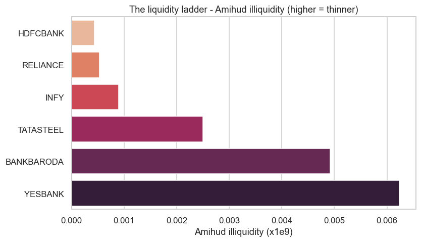
That ladder is a map of where you can deploy capital. A strategy might show a gorgeous backtest on a thin small-cap - until you realise that buying a meaningful position would push the price so far that the edge evaporates. The deep names at the bottom of the ladder can absorb real money; the thin ones at the top are a trap for size.

Liquidity is a cost - and a constraint

So liquidity wears two hats. It's a cost: spread plus impact, paid on every trade. And it's a constraint: it caps how much capital a strategy can hold - its capacity. A quant evaluates both. The most common way retail backtests lie is by ignoring impact and assuming you can trade unlimited size at the last price. You can't. The market charges you for size, every single time.

Try it yourself

• Add a deeply liquid index future (NIFTY...FUT on NFO) and a tiny small-cap to the Amihud basket. How many times more illiquid is the small-cap?
• For your favourite stock, divide its average daily turnover by 100. That rough figure is a sane ceiling on a single order if you want to avoid serious impact - how big is it?
• During market hours, place a hypothetical large order against the live depth() and sum the quantity across levels until it's filled. What average price would you actually get?

Recap

• Liquidity has three faces: spread (immediate cost), depth (size before impact), and resilience (how fast the book refills).
• Trading size moves the price against you - your order walks the book and your average fill is worse than the best quote. That gap is market impact.
• Kyle's lambda is just the price of size - how far price moves per unit of order flow; tiny for liquid names, large for thin ones.
• The Amihud measure (|return| per rupee traded) puts a computable number on illiquidity and ranks the market into a liquidity ladder.
• Liquidity is both a cost and a capacity constraint - ignoring impact is the most common way a backtest flatters a strategy that can't actually be traded.

We've now fully dissected how prices form and what they cost to move. Next we turn to who and what is pushing them - order flow, informed versus uninformed trading, and the FII/DII footprints a quant learns to read.