Portfolio Theory & Its Limits

A single brilliant stock pick is a gamble; a well-built portfolio is a machine. Up to now we've hunted for edges one trade at a time. Module F is about assembling them - combining many positions so that the whole is safer than the sum of its parts, sizing each one correctly, and surviving the rare catastrophe. It starts with an idea so powerful that its discoverer won a Nobel Prize, and so fragile that professionals rarely use it as written. Welcome to portfolio theory.

Risk, return, and the magic of covariance

Here's the counter-intuitive heart of it. A portfolio's return is just the weighted average of its holdings' returns. But its risk is not the weighted average of their risks - it depends on how the assets move relative to each other. Two stocks that zig and zag at different times partly cancel out, so combining them produces a portfolio less volatile than either. The mathematical name for "how they move together" is covariance (or, standardised, correlation), and it is the single most important quantity in portfolio construction.

Diversification: the only free lunch

This isn't theory - it's measurable. Take four very different NSE names, look at each one's volatility, then look at the equal-weight portfolio:

# Diversification: combine assets and portfolio risk falls below the average. A free lunch.
import os
from datetime import datetime, timedelta

import numpy as np
import pandas as pd
from openalgo import api

client = api(
    api_key=os.getenv("OPENALGO_API_KEY", "your_api_key_here"),
    host=os.getenv("OPENALGO_HOST", "http://127.0.0.1:5000"),
)

end = datetime.now().strftime("%Y-%m-%d")
start = (datetime.now() - timedelta(days=730)).strftime("%Y-%m-%d")
syms = ["RELIANCE", "INFY", "HDFCBANK", "ITC"]

rets = pd.DataFrame({s: client.history(symbol=s, exchange="NSE", interval="D",
                                       start_date=start, end_date=end)["close"].pct_change()
                     for s in syms}).dropna()


def ann_vol(x):
    return x.std() * np.sqrt(252) * 100


print("Individual annualised volatility:")
for s in syms:
    print(f"  {s:10s}: {ann_vol(rets[s]):.1f}%")

print(f"\nAverage of the individual vols : {np.mean([ann_vol(rets[s]) for s in syms]):.1f}%")
port = rets @ np.repeat(1 / len(syms), len(syms))          # equal-weight portfolio
print(f"Equal-weight PORTFOLIO vol     : {ann_vol(port):.1f}%   <- lower, because they aren't perfectly correlated")
print("\nThat reduction in risk, for free, is the only genuine free lunch in finance.")

Individual annualised volatility:
  RELIANCE  : 21.3%
  INFY      : 26.9%
  HDFCBANK  : 19.7%
  ITC       : 19.1%

Average of the individual vols : 21.7%
Equal-weight PORTFOLIO vol     : 14.2%   <- lower, because they aren't perfectly correlated

That reduction in risk, for free, is the only genuine free lunch in finance.

Stare at the green bar. Each stock alone carries 19-27% volatility, yet the equal-weight portfolio sits at just 14.2% - lower than any individual holding. You gave up nothing in expected return; you simply combined imperfectly-correlated assets and the risk partly cancelled. That free reduction in risk is, in the famous phrase, the only free lunch in finance - and it's why no quant ever bets everything on one name.

The efficient frontier

If diversification is good, what's the best mix? Simulate thousands of random weightings of a handful of stocks, plot each one's risk against its return, and a striking shape appears:

Copy

# The efficient frontier: thousands of random portfolios, and the best risk-return edge.
import os
from datetime import datetime, timedelta
from pathlib import Path

import matplotlib

matplotlib.use("Agg")
import matplotlib.pyplot as plt
import numpy as np
import pandas as pd
import seaborn as sns
from openalgo import api

client = api(
    api_key=os.getenv("OPENALGO_API_KEY", "your_api_key_here"),
    host=os.getenv("OPENALGO_HOST", "http://127.0.0.1:5000"),
)

end = datetime.now().strftime("%Y-%m-%d")
start = (datetime.now() - timedelta(days=730)).strftime("%Y-%m-%d")
syms = ["RELIANCE", "INFY", "HDFCBANK", "ITC", "TATASTEEL"]
rets = pd.DataFrame({s: client.history(symbol=s, exchange="NSE", interval="D",
                                       start_date=start, end_date=end)["close"].pct_change()
                     for s in syms}).dropna()

mean, cov = rets.mean() * 252, rets.cov() * 252
rng = np.random.default_rng(1)
risk, ret, sharpe = [], [], []
for _ in range(4000):
    w = rng.random(len(syms))
    w /= w.sum()
    pr = w @ mean
    pv = np.sqrt(w @ cov @ w)
    risk.append(pv * 100)
    ret.append(pr * 100)
    sharpe.append(pr / pv)

best = int(np.argmax(sharpe))
sns.set_theme(style="whitegrid")
fig, ax = plt.subplots(figsize=(8, 4.5))
sc = ax.scatter(risk, ret, c=sharpe, cmap="viridis", s=8, alpha=0.6)
ax.scatter(risk[best], ret[best], color="#dc2626", s=120, marker="*", label="max-Sharpe portfolio")
fig.colorbar(sc, label="Sharpe ratio")
ax.set_title("The efficient frontier - 4000 random portfolios of 5 NSE stocks")
ax.set_xlabel("Risk (annualised volatility %)")
ax.set_ylabel("Return (annualised %)")
ax.legend()

out = Path(__file__).with_suffix(".png")
plt.savefig(out, dpi=110, bbox_inches="tight")
print(f"Best Sharpe {sharpe[best]:.2f} at risk {risk[best]:.1f}%, return {ret[best]:.1f}%. Saved {out.name}")

Live output

Best Sharpe 0.17 at risk 20.8%, return 3.6%. Saved 02_efficient_frontier.png

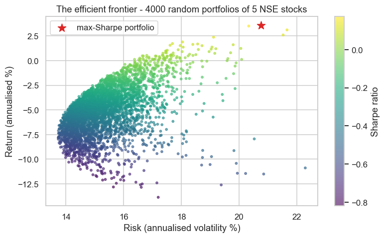
The cloud of portfolios has a hard upper-left edge - the efficient frontier. Any portfolio on that edge gives the maximum possible return for its level of risk; everything below it is sub-optimal (you could earn more for the same risk). The single best point - the brightest in the colour map, marked with a star - is the maximum-Sharpe portfolio, the mix with the best risk-adjusted return. This picture, the efficient frontier, is the founding image of modern portfolio theory.

Mean-variance optimisation

Rather than simulate, you can solve for that best portfolio directly. Mean-variance optimisation (Markowitz) takes your estimated returns and covariances and computes the exact weights that maximise return for a given risk - or maximise the Sharpe ratio outright. It's elegant, it's Nobel-winning, and in its raw form it is almost never used by professionals. Why?

Why it fails live

Because it's an error-maximiser. Mean-variance optimisation demands two inputs: expected returns and the covariance matrix. Both are estimated from past data with enormous uncertainty (Chapter 13's ghost returns). The optimiser, hunting for the best mix, gleefully pours capital into whichever asset's return was over-estimated by noise - producing portfolios that are wildly concentrated, unstable, and that change drastically when you add one more day of data. Feed it slightly wrong numbers (and they're always slightly wrong) and it confidently builds a terrible portfolio.

Practical fixes

Real desks keep the insight of portfolio theory while taming its fragility:

• Equal weight - astonishingly hard to beat, because it makes no fragile return forecast at all.
• Risk parity - weight by risk rather than return, so each holding contributes equally to portfolio volatility (Chapter 25).
• Shrinkage - pull noisy estimates toward a sensible prior, stabilising the covariance matrix.
• Constraints - cap position sizes and ban short weights, so the optimiser can't make insane bets.

The lesson isn't that portfolio theory is wrong - diversification is real and the frontier exists. It's that the naive optimiser is dangerous, and humility about your inputs beats mathematical elegance every time.

Try it yourself

• Add a fifth, very different asset (a commodity like GOLDM...FUT, or an index) to the diversification example. Does portfolio risk fall even further?
• Compute the correlation matrix of your basket. Which pair is most correlated, and which is the best diversifier (lowest correlation)?
• Re-run the efficient frontier on a different two-year window. Does the max-Sharpe portfolio's composition stay stable, or lurch around? (That instability is the error-maximisation problem in action.)

Recap

• A portfolio's return is the weighted average of its holdings', but its risk depends on covariance - how the assets move together.
• Diversification combines imperfectly-correlated assets so risk partly cancels - the equal-weight portfolio (14.2%) was less volatile than every stock in it. The only free lunch.
• The efficient frontier is the set of portfolios giving maximum return per unit of risk; its best point is the maximum-Sharpe portfolio.
• Mean-variance optimisation solves for that point - but in practice it's an error-maximiser that pours capital into noise-inflated estimates.
• Professionals tame it with equal weight, risk parity, shrinkage and constraints - keeping diversification's insight while distrusting fragile inputs.

Diversification told us to spread risk; it didn't tell us what to hold. The next chapter answers that with the handful of deep forces - value, momentum, quality, low-volatility - that actually drive returns: factor models.