Mean Reversion & Cointegration

Here comes the most liberating idea in quantitative trading. So far we've struggled to predict where a price is going - and mostly failed, because price is a random walk. But what if you stop trying to predict price at all, and instead predict the relationship between two prices? Some pairs of assets are tied together by an invisible elastic, and while each one wanders unpredictably, the gap between them reliably snaps back. Trade the gap, not the direction, and the whole game changes. The maths behind this is cointegration, and it powers an entire industry of market-neutral strategies.

A man, a dog, and a stretchy leash

The intuition is best felt, not derived. Picture a man walking his dog through Cubbon Park on a long, stretchy leash:

Where will the man be in five minutes? No idea - he wanders. The dog? No clue either. Each is a random walk. But ask a different question - how far apart are they? - and suddenly you can answer: the leash never lets them drift too far, and when the gap stretches wide, it gently tugs them back together. The two paths are unpredictable; the distance between them is not. That is cointegration in one image.

Cointegration is not correlation

This is the distinction that separates amateurs from quants. Correlation measures whether two things move together day to day - and it's treacherous, because two unrelated assets can be correlated by luck over a stretch, then drift apart forever. Cointegration is deeper and rarer: it means two prices are tethered for the long run, so their spread is stationary (Chapter 14) and mean-reverts. Correlation is a short-term coincidence; cointegration is a structural bond. You can trade only the second one.

Testing for cointegration

Let's find a real tethered pair. Reliance and ONGC are both energy giants, leashed by the same oil price - let's test them with the Engle-Granger cointegration test:

# Cointegration: two prices wander, but their SPREAD snaps back. Test and measure it.
import os
from datetime import datetime

import pandas as pd
import statsmodels.api as sm
from openalgo import api
from statsmodels.tsa.stattools import coint

client = api(
    api_key=os.getenv("OPENALGO_API_KEY", "your_api_key_here"),
    host=os.getenv("OPENALGO_HOST", "http://127.0.0.1:5000"),
)

end = datetime.now().strftime("%Y-%m-%d")


def close(symbol):
    return client.history(symbol=symbol, exchange="NSE", interval="D",
                          start_date="2021-01-01", end_date=end)["close"]


df = pd.concat([close("RELIANCE"), close("ONGC")], axis=1).dropna()
df.columns = ["RELIANCE", "ONGC"]
a, b = df["RELIANCE"], df["ONGC"]

pval = coint(a, b)[1]                                   # Engle-Granger test
hedge = sm.OLS(a, sm.add_constant(b)).fit().params.iloc[1]
spread = a - hedge * b
z_now = (spread.iloc[-1] - spread.mean()) / spread.std()

print("Engle-Granger cointegration: RELIANCE vs ONGC")
print(f"  p-value          : {pval:.3f}  -> {'COINTEGRATED (spread mean-reverts)' if pval < 0.05 else 'not cointegrated'}")
print(f"  hedge ratio      : {hedge:.2f}   (1 RELIANCE hedged with {hedge:.2f} ONGC)")
print(f"  spread z-score   : {z_now:+.2f}   ({'stretched - reversion likely' if abs(z_now) > 1.5 else 'near fair value'})")
print("\nCorrelation says they move together; cointegration says their SPREAD reliably comes back.")

Engle-Granger cointegration: RELIANCE vs ONGC
  p-value          : 0.011  -> COINTEGRATED (spread mean-reverts)
  hedge ratio      : 2.58   (1 RELIANCE hedged with 2.58 ONGC)
  spread z-score   : -0.36   (near fair value)

Correlation says they move together; cointegration says their SPREAD reliably comes back.

A p-value of 0.011 clears the bar - these two are genuinely cointegrated, their spread mean-reverts. The hedge ratio of 2.58 is the recipe for the trade: to make the spread market-neutral, you pair 1 unit of Reliance against 2.58 units of ONGC, so that broad market moves cancel out and only the relationship remains. Right now the spread's z-score is near zero - fair value, no trade. But when it stretches...

The spread and its z-score

...you get a signal. Convert the spread to a z-score - how many standard deviations it sits from its own mean - and the strategy writes itself:

Copy

# The spread's z-score is the pairs-trading signal: short the highs, buy the lows.
import os
from datetime import datetime
from pathlib import Path

import matplotlib

matplotlib.use("Agg")
import matplotlib.pyplot as plt
import pandas as pd
import seaborn as sns
import statsmodels.api as sm
from openalgo import api

client = api(
    api_key=os.getenv("OPENALGO_API_KEY", "your_api_key_here"),
    host=os.getenv("OPENALGO_HOST", "http://127.0.0.1:5000"),
)

end = datetime.now().strftime("%Y-%m-%d")


def close(symbol):
    return client.history(symbol=symbol, exchange="NSE", interval="D",
                          start_date="2021-01-01", end_date=end)["close"]


df = pd.concat([close("RELIANCE"), close("ONGC")], axis=1).dropna()
df.columns = ["RELIANCE", "ONGC"]
hedge = sm.OLS(df["RELIANCE"], sm.add_constant(df["ONGC"])).fit().params.iloc[1]
spread = df["RELIANCE"] - hedge * df["ONGC"]
z = (spread - spread.mean()) / spread.std()

sns.set_theme(style="whitegrid")
fig, ax = plt.subplots(figsize=(8, 4.5))
ax.plot(z.index, z, color="#7c83ff", lw=1)
ax.axhline(0, color="#555", lw=1)
ax.axhline(2, color="#dc2626", ls="--", lw=1.4, label="+/-2 sigma (entry)")
ax.axhline(-2, color="#16a34a", ls="--", lw=1.4)
ax.fill_between(z.index, 2, z, where=(z > 2), color="#dc2626", alpha=0.25)
ax.fill_between(z.index, -2, z, where=(z < -2), color="#16a34a", alpha=0.25)
ax.set_title("RELIANCE - ONGC spread z-score (short red, buy green, exit at 0)")
ax.set_ylabel("Z-score of the spread")
ax.legend()

out = Path(__file__).with_suffix(".png")
plt.savefig(out, dpi=110, bbox_inches="tight")
print(f"Spread crossed +/-2 sigma on {int((z.abs() > 2).sum())} days - each a potential pairs trade. Saved {out.name}")

Live output

Spread crossed +/-2 sigma on 43 days - each a potential pairs trade. Saved 02_spread_zscore.png

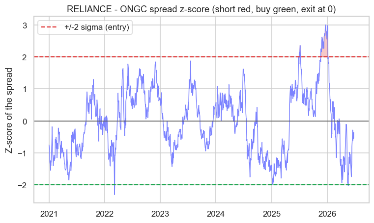
Read the bands: when the z-score spikes above +2 (red), the spread is unusually stretched, so you short it (sell Reliance, buy ONGC) and wait for the snap back. When it drops below −2 (green), you buy the spread. You exit as it crosses zero - back at fair value. Over this window the spread hit those bands on 43 days, each a textbook pairs-trade opportunity. You never once needed an opinion on where the market was heading.

Mean reversion and the half-life

Mathematically the spread behaves like an Ornstein-Uhlenbeck process - the formal name for "a random walk on a leash," a series constantly pulled back toward its mean with a measurable strength. From that pull you can estimate the half-life: how long, on average, the spread takes to close half the distance back to fair value. A short half-life means quick, frequent trades; a long one means patience. It's the single most useful number for setting your holding period and deciding whether a pair is even worth trading.

Why this is so powerful - and its danger

The beauty is market neutrality: a pairs trade is long one asset and short another, so a market-wide crash or rally largely cancels out. Your profit comes purely from the spread reverting, which makes the strategy's returns nearly independent of the index - gold dust for a diversified book (Module G's statistical arbitrage).

Try it yourself

• Re-run the test on HDFCBANK vs ICICIBANK. Are two big private banks cointegrated, or just correlated? (You may be surprised how often "obvious" pairs fail.)
• Estimate the half-life of the Reliance-ONGC spread by regressing its daily change on its lagged level. Is it days or weeks?
• Split the history in two and test cointegration on each half separately. Does the relationship hold in both, or did the leash stretch over time?

Recap

• Stop predicting price; predict the relationship. Some pairs are tied by an elastic leash - each wanders, but their spread mean-reverts.
• Cointegration (a stationary, mean-reverting spread) is a deep structural bond - utterly different from correlation, which is a fragile short-term coincidence.
• The Engle-Granger test confirms a pair (Reliance-ONGC, p = 0.011); the hedge ratio (2.58) builds a market-neutral spread.
• The spread's z-score is the signal: short above +2σ, buy below −2σ, exit at zero - 43 opportunities in this window, with no market view needed.
• The spread is an Ornstein-Uhlenbeck process; its half-life sets your holding period - and because a leash can snap, every pairs trade needs a stop and a re-test.

We've modelled volatility and relationships - the two things that genuinely mean-revert. The last piece of Module D is recognising when the rules change entirely: market regimes and the structural breaks that quietly kill a working strategy.