Cross-Sectional Momentum & Value

Two strategies have driven systematic equity investing for decades: momentum (buy what's been rising) and value (buy what's cheap). Unlike the pairs trade, these take a directional view - but a disciplined, systematic, cross-sectional one. Instead of asking "will this stock go up?", they ask "which stocks are best relative to their peers?" - rank the whole universe, buy the top, short the bottom. This chapter builds that long-short machine, and - true to our honesty rule - lets the Indian data say something uncomfortable about when these factors actually work.

Cross-sectional versus time-series

First, a crucial distinction. A time-series signal looks at one asset's own history - "is Nifty trending up?" A cross-sectional signal compares assets to each other - "which stocks have the strongest momentum relative to the rest?" Cross-sectional strategies don't care if the whole market is up or down; they care about the spread between the best and worst names. Rank the universe, go long the leaders and short the laggards, and you've built a market-neutral factor bet.

Building the long-short

Here's the machine. Every month, rank our universe of NSE stocks by their trailing 6-month return, buy the top third, short the bottom third, hold for a month, then rebalance:

# Cross-sectional momentum: each month, go long the winners and short the losers.
import os
from datetime import datetime

import numpy as np
import pandas as pd
from openalgo import api

client = api(
    api_key=os.getenv("OPENALGO_API_KEY", "your_api_key_here"),
    host=os.getenv("OPENALGO_HOST", "http://127.0.0.1:5000"),
)

end = datetime.now().strftime("%Y-%m-%d")
universe = ["RELIANCE", "INFY", "HDFCBANK", "ITC", "TATASTEEL", "ADANIENT", "SBIN",
            "BHARTIARTL", "MARUTI", "SUNPHARMA", "TITAN", "HINDALCO", "AXISBANK",
            "LT", "WIPRO", "POWERGRID"]

prices = pd.DataFrame({s: client.history(symbol=s, exchange="NSE", interval="D",
                                         start_date="2021-01-01", end_date=end)["close"]
                       for s in universe})

monthly = prices.resample("ME").last()
momentum = monthly.pct_change(6)            # 6-month return = the ranking signal
forward = monthly.pct_change().shift(-1)    # next month's return = the test

ls = []
for date in momentum.index:
    score = momentum.loc[date].dropna()
    if len(score) < 6:
        continue
    n = len(score) // 3
    winners, losers = score.nlargest(n).index, score.nsmallest(n).index
    ls.append(forward.loc[date, winners].mean() - forward.loc[date, losers].mean())

ls = pd.Series(ls).dropna()
print(f"Cross-sectional momentum (long winners, short losers), monthly rebalance:")
print(f"  Avg monthly long-short return : {ls.mean() * 100:+.2f}%")
print(f"  Win rate (positive months)    : {(ls > 0).mean() * 100:.0f}%")
print(f"  Annualised Sharpe             : {ls.mean() / ls.std() * np.sqrt(12):+.2f}")
print("\nSign and strength depend on the regime - momentum and reversal trade places over time.")

Cross-sectional momentum (long winners, short losers), monthly rebalance:
  Avg monthly long-short return : -0.94%
  Win rate (positive months)    : 47%
  Annualised Sharpe             : -0.67

Sign and strength depend on the regime - momentum and reversal trade places over time.

The honest result

And here's where the data refuses to flatter us. The momentum long-short produced a negative return and a Sharpe of −0.67 over this window. Sort the stocks into groups and the pattern is the opposite of what momentum predicts:

Copy

# Sort stocks into groups by momentum, then check each group's next-month return.
import os
from datetime import datetime
from pathlib import Path

import matplotlib

matplotlib.use("Agg")
import matplotlib.pyplot as plt
import numpy as np
import pandas as pd
import seaborn as sns
from openalgo import api

client = api(
    api_key=os.getenv("OPENALGO_API_KEY", "your_api_key_here"),
    host=os.getenv("OPENALGO_HOST", "http://127.0.0.1:5000"),
)

end = datetime.now().strftime("%Y-%m-%d")
universe = ["RELIANCE", "INFY", "HDFCBANK", "ITC", "TATASTEEL", "ADANIENT", "SBIN",
            "BHARTIARTL", "MARUTI", "SUNPHARMA", "TITAN", "HINDALCO", "AXISBANK",
            "LT", "WIPRO", "POWERGRID"]

prices = pd.DataFrame({s: client.history(symbol=s, exchange="NSE", interval="D",
                                         start_date="2021-01-01", end_date=end)["close"]
                       for s in universe})
monthly = prices.resample("ME").last()
momentum = monthly.pct_change(6)
forward = monthly.pct_change().shift(-1)

GROUPS = 4
bucket_ret = {g: [] for g in range(GROUPS)}
for date in momentum.index:
    score = momentum.loc[date].dropna()
    if len(score) < GROUPS:
        continue
    ranks = score.rank()
    labels = pd.qcut(ranks, GROUPS, labels=False)
    for g in range(GROUPS):
        names = labels[labels == g].index
        bucket_ret[g].append(forward.loc[date, names].mean())

avg = [np.nanmean(bucket_ret[g]) * 100 for g in range(GROUPS)]
names = ["Q1\n(losers)", "Q2", "Q3", "Q4\n(winners)"]

sns.set_theme(style="whitegrid")
fig, ax = plt.subplots(figsize=(8, 4.5))
sns.barplot(x=names, y=avg, hue=names, legend=False, palette="viridis", ax=ax)
ax.axhline(0, color="#555", lw=1)
ax.set_title("Next-month return by momentum group (monotonic rise = momentum works)")
ax.set_ylabel("Avg next-month return (%)")
out = Path(__file__).with_suffix(".png")
plt.savefig(out, dpi=110, bbox_inches="tight")
print(f"Group returns (low->high momentum): {[round(float(a), 2) for a in avg]}. Saved {out.name}")

Live output

Group returns (low->high momentum): [1.49, 1.84, 0.91, 0.7]. Saved 02_quintile_returns.png

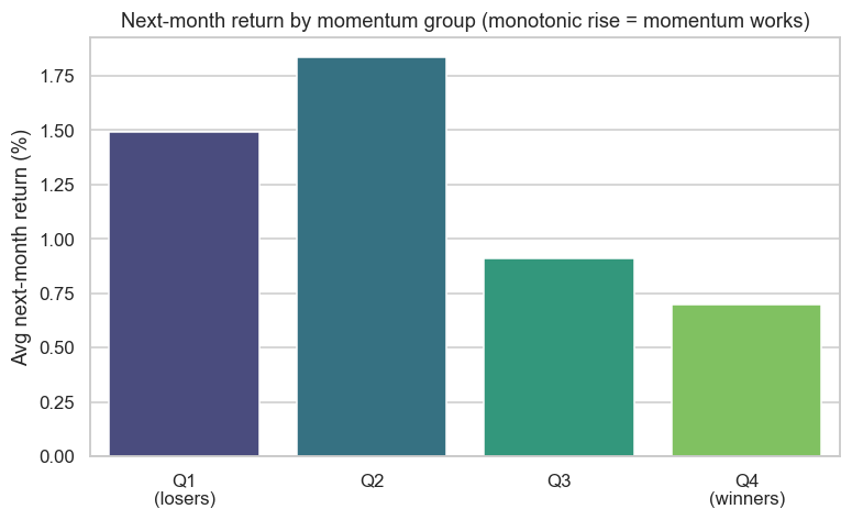
The group returns run roughly downhill, not uphill - the recent losers outperformed the recent winners. In this period and this universe, the Indian market showed short-term reversal, not momentum. We're not going to hide that behind a cherry-picked window. The method is exactly right and is what you're learning; the sign of the edge depended entirely on the regime - precisely the lesson of Chapters 24 and 27.

Horizon matters

So is momentum fake? No - the subtlety is horizon. The same prices behave differently at different time scales: over days to a few weeks markets tend to reverse (overreactions snap back); over 3 to 12 months they tend to trend (true momentum); over 3 to 5 years they revert again (the long-horizon value effect). Our 6-month-formation, 1-month-hold test sat in a zone where, for this recent Indian window, reversal won. Pick the wrong horizon - or the wrong regime - and momentum becomes its own opposite. The professional builds the signal at the horizon where the effect is documented and robust, and re-tests it relentlessly.

Value: the other workhorse

Value is momentum's natural partner. Rather than ranking by recent return, rank by cheapness - low price-to-earnings, low price-to-book - and buy the cheap, short the dear. Over long horizons and broad universes, cheap stocks have historically beaten expensive ones, a premium for the discomfort of owning unloved names. Value and momentum are famously negatively correlated - value loves the beaten-down stocks momentum is shorting - which is exactly why combining them is so powerful.

Combining factors

Which is the real lesson of this chapter. No single factor is reliable - we just watched momentum invert. But blend several lowly-correlated factors (momentum, value, quality, low-vol from Chapter 24) into one composite score, rank on that, and hold across a broad universe for a long horizon, and the ensemble is far steadier than any component. When momentum is having a terrible year (like this one), value or quality often carries the book. Multi-factor, diversified, patient - that's how systematic equity actually survives.

Try it yourself

• Flip the signal: go long the losers and short the winners (a reversal strategy). In this window, does the sign flip turn the −0.67 Sharpe positive?
• Change the formation window from 6 months to 12. Does longer-horizon momentum behave differently from the short-horizon version?
• Expand the universe from 16 stocks to a full Nifty-50 list. Does a broader cross-section make the factor steadier (less noise)?

Recap

• Cross-sectional strategies rank assets against each other and trade the spread - long the best, short the worst - a market-neutral factor bet.
• The long-short machine: rank the universe, buy the top, short the bottom, rebalance periodically.
• Honestly, cross-sectional momentum reversed in this Indian window (Sharpe −0.67; group returns ran downhill) - factors are regime-dependent.
• Horizon matters: short term reverses, intermediate term trends, long term reverts - the same prices give opposite signals at different scales.
• Value is momentum's negatively-correlated partner; the robust answer is a diversified, multi-factor, long-horizon book where one factor's drought is another's feast.

Momentum and value are systematic directional bets. The next family is sharper and more event-specific: trading the calendar and the flows - earnings, index rebalancing, expiry effects and FII activity.