
Example scripts
Twelve complete OpenScript files, from an EMA cross to a short options premium strategy, and three showcase studies, each explained with what it shows on the chart and where it runs in /trading.
On this page
- The twelve at a glance
- Where they run in /trading today
- 1. EMA cross
- 2. Trailing volatility stop
- 3. Anchored VWAP
- 4. RSI divergence
- 5. Opening range
- 6. Combined premium
- 7. Higher timeframe bias
- 8. Dashboard
- 9. Supply and demand zones
- 10. EMA cross, bracketed
- 11. Opening range breakout
- 12. Short premium, combined stop
- Showcase scripts
These twelve scripts are complete files you can paste into the Scripts panel, save and apply. Each one is small enough to read in a few minutes and makes one or two ideas of the language concrete: nine are studies and three are strategies, and they run from a first EMA cross to a two leg options premium strategy. For every script, this page says what it draws, which language features it shows and why they are written the way they are, and where it runs in /trading today. After them, Showcase scripts gives three studies written to look their best on a chart, each with the screenshot it drew.
The comments inside each script say why a line is written the way it is, not what it does. For what a function does, follow its link to the reference.
The twelve at a glance
| # | Script | Kind | Shows |
|---|---|---|---|
| 1 | EMA cross | Study | Inputs, two averages, a shaded band and a crossing marker |
| 2 | Trailing volatility stop | Study | Values carried between bars with var, orElse(), bar colouring |
| 3 | Anchored VWAP | Study | A time input, running totals, absence as "not started yet" |
| 4 | RSI divergence | Study | Pivots and their lag, lines and labels drawn between two past points |
| 5 | Opening range | Study | The session's first bar, state that resets each day, background shading |
| 6 | Combined premium | Study | Reading two option contracts that are not on the chart, and an alert |
| 7 | Higher timeframe bias | Study | A daily reading on an intraday chart, stated so it cannot repaint |
| 8 | Dashboard | Study | A table fixed to a corner, a user function, switch |
| 9 | Supply and demand zones | Study | Boxes created, extended and deleted over hundreds of bars |
| 10 | EMA cross, bracketed | Strategy | Costs, a stop and a target fixed at entry, risk-based sizing |
| 11 | Opening range breakout | Strategy | One trade per session, the range as the stop, an exit on the clock |
| 12 | Short premium, combined stop | Strategy | Two legs managed as one position on their combined price |
Where they run in /trading today
Every script here compiles with no error. A few use features the /trading page does not supply to the engine yet, and it is better to know that before you apply one than to wonder why it drew nothing.
| Script | On the chart | Backtest panel | Strategies panel |
|---|---|---|---|
| 1, 2, 4, 7, 8, 9 | Draws as described | Not a strategy | Not a strategy |
| 3 Anchored VWAP | Draws as described, with the anchor time read as UTC | Not a strategy | Not a strategy |
| 5 Opening range | Draws nothing yet: needs the session's opening time | Not a strategy | Not a strategy |
| 6 Combined premium | Draws the premium; two parts need facts the chart does not state yet | Not a strategy | Not a strategy |
| 10 EMA cross, bracketed | Draws and simulates its trades | Runs. Its exit() levels are not filled, so trades close on the opposite cross | Refused: it calls exit() |
| 11 Opening range breakout | Opens no trades: needs the session's opening time | Opens no trades, for the same reason | Refused: it reads the session, calls exit() and sizes in lots |
| 12 Short premium | Draws the premium, opens no trades: needs the session | Refused with OS6006: it reads another instrument | Refused: it reads the session, the calendar and another instrument, and sizes in lots |
| Showcase: HalfTrend, Bollinger Bands, EMA cross in colour | Draws as described | Not a strategy | Not a strategy |
The notes under each script explain the reason. Your first strategy builds a strategy that runs in all three places.
1. EMA cross
The script every reader meets first, and the one the Quickstart builds. Two exponential moving averages (ema()), the band between them shaded with fill(), and a signal() marker on each bar where they cross. It works on any instrument and any timeframe.
// Two exponential moving averages, the band between them, and a marker on the
// bar where they cross.
//
// The crossing is a signal() rather than a plotted value, because a crossing is
// an event on one bar, not a number on every bar.

version 1

study("EMA cross", overlay = true, precision = 2)

fastLen = input(9,  "Fast length", min = 1, max = 500)
slowLen = input(21, "Slow length", min = 1, max = 500)
src     = input(close, "Source")

fast = ema(src, fastLen)
slow = ema(src, slowLen)

// Both crosses are computed at the top level, on every bar. Computed inside the
// branch that uses them, they would advance only on the bars that branch runs,
// which is warning OS8001 and a missed crossing.
up   = crossUp(fast, slow)
down = crossDown(fast, slow)

// fill() shades between two plots, and takes the plots themselves rather than
// the series they draw, so both plots are named.
fastPlot = plot(fast, "Fast", aqua, width = 2)
slowPlot = plot(slow, "Slow", orange, width = 2)

// The band inherits the warmup of the two lines it joins: neither average has a
// value before its window fills, so the fill simply starts where they do.
fill(fastPlot, slowPlot, fade(aqua, 90))

if up
    signal("BUY")

if down
    signal("SELL")
A version dressed for the chart, with 20 and 50 bar averages, the band coloured by which one leads and each crossing labelled, is EMA cross in colour under Showcase scripts, with its screenshot.
What to notice:
- The ordinary case is short. No namespace on
ema, no prefix onaqua, and onesignal("BUY")for a marker. - Stateful calls live at the top level.
crossUp()andcrossDown()compare this bar with the previous one, so they must see every bar. The script computes them first and tests the result inside theif. - A band belongs to two plots.
plot()returns a handle when you name it, andfill()takes two handles. Passing an expression instead of a plot is OS3020. input(close, "Source")gives the settings dialog a menu of price series, so the same study can average the typical price (hlc3) without an edit.
2. Trailing volatility stop
A band that trails price at a multiple of the average true range (atr()), flips side when price closes through it, and recolours the candles by direction. It is built by hand to show two ideas at work: values carried from one bar to the next with var, and orElse() supplying a starting value where the past does not exist yet. The library's own supertrend() computes the same kind of band in one call.
// A trailing volatility stop: the two raw bands it is built from, the one band
// in force, and the price candles recoloured by which side price is on.

version 1

study("Trailing volatility stop", overlay = true, precision = 2)

atrLen = input(10,  "ATR length", min = 1, max = 200)
mult   = input(3.0, "Band width, in ATR", min = 0.5, max = 20)
paint  = input(true, "Recolour the candles")

atrValue = atr(atrLen)

// The raw bands, recomputed from scratch every bar. The trailing bands are
// pulled towards them.
rawLower = hl2 - mult * atrValue
rawUpper = hl2 + mult * atrValue

var lowerBand = none
var upperBand = none
var dir = 1

// Read the two bands before they are reassigned below. At this point in the
// file a var still holds the previous bar's value, so no [1] read is needed.
prevLower = lowerBand
prevUpper = upperBand

// Until the ATR has warmed up there is no previous band, and max and min pass
// absence through like any other calculation. Trailing against an absent band
// would leave the band absent for the rest of the chart, because each bar
// trails the one before. So the previous band falls back to the raw band.
heldLower = orElse(prevLower, rawLower)
heldUpper = orElse(prevUpper, rawUpper)

lowerBand = close[1] > heldLower ? max(rawLower, heldLower) : rawLower
upperBand = close[1] < heldUpper ? min(rawUpper, heldUpper) : rawUpper

// The direction flips against the band as it stood on the previous bar, not the
// band this bar just produced, or every bar would trigger its own flip.
if not isNone(prevUpper) and close > prevUpper
    dir = 1
else if not isNone(prevLower) and close < prevLower
    dir = -1

stopLine = dir == 1 ? lowerBand : upperBand

// Two plots rather than one, each with a gap where the other is in force, so a
// flip jumps cleanly instead of drawing a diagonal from one side to the other.
plot(dir ==  1 ? stopLine : none, "Stop, long",  lime, width = 2)
plot(dir == -1 ? stopLine : none, "Stop, short", red,  width = 2)

upperPlot = plot(rawUpper, "Upper band", fade(silver, 60))
lowerPlot = plot(rawLower, "Lower band", fade(silver, 60))
fill(upperPlot, lowerPlot, fade(silver, 94))

barColor(paint ? (dir == 1 ? lime : red) : none)

// bar.isFirst guards the flip test: on bar 0 the previous direction is absent,
// dir != dir[1] is true, and the study would mark a flip that never happened.
if not bar.isFirst and dir != dir[1]
    signal(dir == 1 ? "TREND UP" : "TREND DOWN")
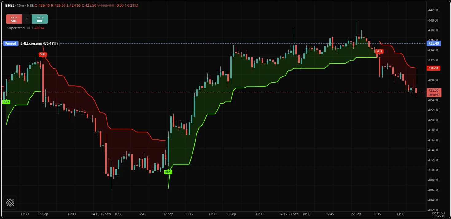
The same kind of trailing band on a BHEL 15 minute chart, from a Supertrend study with a 10 bar ATR and a multiplier of 3 that shades between the band and the candles and labels each flip BUY or SELL:
What to notice:
varremembers.var lowerBand = noneis set once, on the first bar, and then keeps its value from bar to bar. Read before it is reassigned, it still holds the previous bar's value. See Persistence.- Absence travels.
max()andmin()of an absent value are absent. WithoutorElse(), one absent start would make the band absent forever. See Absent values. - A plot is hidden with
none. Each stop line is givennoneon the bars where the other side is in force. barColor()repaints the candles, and gives them back their own colour when handednone.
3. Anchored VWAP
The volume weighted average price measured from a date and time you choose, with standard deviation bands around it. On an NSE chart, anchor it at a results day, a budget day or the start of the month, and it shows the average price paid by everyone who traded since.
// Volume weighted average price measured from a date and time you pick, with
// standard deviation bands around it.

version 1

study("Anchored VWAP", overlay = true, precision = 2)

anchorTime = input("2025-01-01 09:15", "Anchor", kind = "time")
src        = input(hlc3, "Source")
bandMult   = input(1.0, "Band width, in standard deviations", min = 0.1, max = 5)
showBands  = input(true, "Show the bands")

// A time input is typed as a date and a clock time, and reads in the script as
// a timestamp that compares directly with time. An anchor that cannot be read
// is absent: the comparison below is then absent on every bar, nothing
// accumulates, and the plot is empty rather than wrong.

var priceVolume  = 0.0
var squareVolume = 0.0
var totalVolume  = 0.0
var started      = false

if not started and time >= anchorTime
    started = true

// Three running sums rather than a list of every bar since the anchor. The
// newest bar is recomputed as each update arrives, and every var is restored to
// its previous bar's value before each recompute, so the sums count bars and
// not updates.
if started
    priceVolume  += src * volume
    squareVolume += src * src * volume
    totalVolume  += volume

// vwap and variance are library names, and assigning to one is OS2002, so the
// two readings computed here have names of their own.
ready     = started and totalVolume > 0
vwapValue = ready ? priceVolume / totalVolume : none

// Rounding can leave the variance very slightly below zero on a long run of
// near identical prices. It is floored at zero before the square root; without
// the floor, sqrt would return none and leave a one bar hole in both bands.
varianceValue = ready ? max(squareVolume / totalVolume - vwapValue * vwapValue, 0) : none
dev           = ready ? sqrt(varianceValue) : none

upper = showBands ? vwapValue + bandMult * dev : none
lower = showBands ? vwapValue - bandMult * dev : none

plot(vwapValue, "Anchored VWAP", orange, width = 2)
// With the bands switched off, both edges are absent on every bar, so the fill
// stops with them and needs no test of its own.
upperPlot = plot(upper, "Upper band", aqua)
lowerPlot = plot(lower, "Lower band", aqua)
fill(upperPlot, lowerPlot, fade(aqua, 92))

// Mark the anchor bar. orElse is needed on bar 0, where started[1] is absent:
// an absent condition takes the false branch, so an anchor on the very first
// bar would otherwise go unmarked.
if started and not orElse(started[1], false)
    signal("ANCHOR")
What to notice:
kind = "time"makes the input a date and time field. In the study's settings dialog it is a text box in the formYYYY-MM-DD HH:MM.- Running totals in
varare safe on a chart that is still receiving ticks, because the newest bar is rolled back and recomputed rather than counted twice. See Realtime and confirmation. - Absence means "not started". Before the anchor,
readyis false and every reading isnone, so nothing is drawn. sqrt()of a negative number returnsnonerather than failing. The script floors the value withmax()instead of relying on that.
4. RSI divergence
Regular divergence between price and the relative strength index (rsi()): a line drawn between two RSI pivots when the oscillator disagrees with the price extremes under them. A pivot is a turning point: a bar whose value is the highest (or lowest) of a few bars on each side of it. Divergence is price and the oscillator moving in opposite directions between two pivots. A higher high in price with a lower high in RSI is marked bearish; a lower low with a higher low is marked bullish.
// Regular divergence between price and an oscillator: a line drawn between the
// two oscillator pivots that disagree with the two price extremes under them.

version 1

study("RSI divergence", precision = 2, range = [0, 100])

rsiLen    = input(14, "RSI length", min = 2, max = 200)
leftBars  = input(5,  "Pivot left bars",  min = 1, max = 50)
rightBars = input(5,  "Pivot right bars", min = 1, max = 50)
maxSpan   = input(60, "Longest divergence, in bars", min = 5, max = 500)

oscillator = rsi(close, rsiLen)

level(70, "Overbought", fade(red, 50))
level(50, "Middle", fade(gray, 60))
level(30, "Oversold", fade(lime, 50))
plot(oscillator, "RSI", purple, width = 2)

// A pivot is only known rightBars bars after the bar it happened on, so every
// value this study reads is offset by that much. That lag is the honest cost of
// a pivot: the marker appears late because the pivot could not be known sooner.
pivotUp   = pivotHigh(oscillator, leftBars, rightBars)
pivotDown = pivotLow(oscillator, leftBars, rightBars)

var lastHighOsc   = none
var lastHighPrice = none
var lastHighTime  = none
var lastHighBar   = none

var lastLowOsc   = none
var lastLowPrice = none
var lastLowTime  = none
var lastLowBar   = none

if not isNone(pivotUp)
    thisPrice = high[rightBars]
    thisTime  = time[rightBars]
    thisBar   = bar.index - rightBars
    // Both bar indices come from the same run, so their difference is a real
    // bar count. The drawing is anchored to the time, because loading older
    // history renumbers every bar index and would drag the line sideways.
    known  = not isNone(lastHighBar)
    nearby = known and thisBar - lastHighBar <= maxSpan
    if nearby and thisPrice > lastHighPrice and pivotUp < lastHighOsc
        draw.line(lastHighTime, lastHighOsc, thisTime, pivotUp, color = red, width = 2)
        draw.label(thisTime, pivotUp, "Bearish", color = red, textColor = white)
        signal("BEARISH")
    lastHighOsc   = pivotUp
    lastHighPrice = thisPrice
    lastHighTime  = thisTime
    lastHighBar   = thisBar

if not isNone(pivotDown)
    thisPrice = low[rightBars]
    thisTime  = time[rightBars]
    thisBar   = bar.index - rightBars
    known  = not isNone(lastLowBar)
    nearby = known and thisBar - lastLowBar <= maxSpan
    if nearby and thisPrice < lastLowPrice and pivotDown > lastLowOsc
        draw.line(lastLowTime, lastLowOsc, thisTime, pivotDown, color = lime, width = 2)
        draw.label(thisTime, pivotDown, "Bullish", color = lime, textColor = black)
        signal("BULLISH")
    lastLowOsc   = pivotDown
    lastLowPrice = thisPrice
    lastLowTime  = thisTime
    lastLowBar   = thisBar
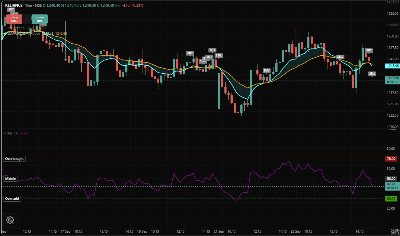
Without overlay = true, the study gets its own pane under the price, and range = [0, 100] pins that pane's scale so the three levels stay put. Here is an RSI pane with the same three levels:
What to notice:
- Pivots arrive late, visibly.
pivotHigh()andpivotLow()return a valuerightBarsbars after the turn, because only then is it known. The script readshigh,lowandtimerightBarsbars back to find the turning bar. - Drawings anchor to time.
draw.line()anddraw.label()take a bar time, not a bar index, because an index shifts when older history loads. See Lines and boxes. - Block scope.
thisPriceinside the firstifandthisPriceinside the second are two separate names that exist only in their blocks. level()draws the 70, 50 and 30 reference lines.
5. Opening range
The high and low of the first minutes of each session, held for the rest of the day, with the first break of either side marked once. On NSE, where the session opens at 09:15 IST, the default 15 minute range covers 09:15 to 09:30.
// The high and low of the first minutes of each session, held for the rest of
// the day, with the first break of either side marked once.

version 1

study("Opening range", overlay = true, precision = 2)

rangeMinutes = input(15, "Opening range, in minutes", min = 1, max = 240)
shadeOpacity = input(1,  "Shading opacity, 0 turns the shading off",
                     min = 0, max = 1)

var openTime  = none
var rangeHigh = none
var rangeLow  = none
var broken    = 0

// Everything resets on the session's first bar rather than on a change of date,
// because a session is what an exchange opens: an evening session that runs
// past midnight is one session and two dates.
if session.isFirstBar
    openTime  = time
    rangeHigh = high
    rangeLow  = low
    broken    = 0

// Milliseconds since the open rather than a clock comparison, so the script
// says the same thing in any time zone and needs no calendar.
elapsed = isNone(openTime) ? none : time - openTime
forming = not isNone(elapsed) and elapsed < rangeMinutes * 60000

if forming and not session.isFirstBar
    rangeHigh = max(rangeHigh, high)
    rangeLow  = min(rangeLow, low)

// The first break of either side, once per session. broken is a number rather
// than a bool, so it also records which side broke.
if not forming and broken == 0 and not isNone(rangeHigh)
    if close > rangeHigh
        broken = 1
        signal("BREAK UP")
    else if close < rangeLow
        broken = -1
        signal("BREAK DOWN")

highPlot = plot(rangeHigh, "Range high", aqua,   width = 2, style = "step")
lowPlot  = plot(rangeLow,  "Range low",  orange, width = 2, style = "step")

// The shading switch is an opacity of zero, not a colour of none: fill() reads
// an absent colour as "no colour given" and shades with a default. opacity dims
// whatever colour is there, and zero is off. It is a number input because
// opacity is settled before the first bar and takes a number from 0 to 1.
fill(highPlot, lowPlot, fade(aqua, 93), opacity = shadeOpacity)

// A background rather than a fourth line, because "the range is still forming"
// is a fact about the whole bar and has no price to sit at.
background(forming ? fade(silver, 92) : none)
What to notice:
session.isFirstBaris true on the first bar of each trading session. Resetting state there, instead of on a change of date, is what makes the script right for MCX's evening session as well as NSE's day session. See Sessions and time.- Time arithmetic in milliseconds.
timeis a timestamp in milliseconds, sorangeMinutes * 60000is the length of the range. style = "step"draws a level that changes in steps rather than sloping between bars.background()shades the bars while the range is forming.
6. Combined premium
The combined price of two option legs, such as the call and put of a NIFTY straddle on NFO (a call and a put at the same strike and expiry), read from two contracts that are not on the chart, with the session's opening premium held as a reference and an alert when the premium has decayed by a chosen percentage.
// The combined price of two option legs, read from two instruments that are not
// the one on the chart, with the session's opening premium held as a reference.

version 1

study("Combined premium", precision = 2, format = "price")

// Plain text inputs: type each leg's trading symbol. An instrument picker input
// is planned, and until it exists the legs are typed in.
callLeg   = input("", "Call leg")
putLeg    = input("", "Put leg")
lots      = input(1,  "Lots", min = 1, max = 100)
targetPct = input(30, "Decay to mark, in percent of the opening premium", min = 1, max = 99)

// Each leg is read at the chart's own interval and aligned to the chart's bars,
// so the sum below adds two prices from the same moment. The read uses the
// default mode, "confirmed", which never repaints.
callPrice = req.symbol(callLeg, chart.interval, close, exchange = chart.exchange)
putPrice  = req.symbol(putLeg,  chart.interval, close, exchange = chart.exchange)

// If either leg has no bar at this time, the sum is absent, not half a
// position. A missing leg shows as a gap in the line instead of a smaller
// number that looks like a profit.
premium = callPrice + putPrice
money   = premium * lots * chart.lotSize

var opening = none

if session.isFirstBar
    opening = none

if isNone(opening) and not isNone(premium)
    opening = premium

// Decay is positive when the seller of both legs is ahead, which is the sign a
// premium seller expects, so the subtraction is written that way round.
decay = isNone(opening) ? none : (opening - premium) / opening * 100

plot(premium, "Combined premium", orange, width = 2)
plot(opening, "Opening premium", fade(silver, 40), style = "step")
plot(money,   "Position value", aqua, scale = "left")

// The condition is the if around the call, not an argument to alert(). decay is
// absent on any bar where either leg is missing, and an absent condition takes
// the false branch, so neither the alert nor the marker fires on a gap.
if decay >= targetPct
    alert("Combined premium decayed " + text(decay, 1) + " percent",
          id = "premium-decay")
    signal("TARGET")
To use it, open a chart on NFO, for example the NIFTY future or one of the two legs, and type both legs' trading symbols into the study's settings. Both legs are read on the chart's own exchange and at the chart's own interval.
What to notice:
req.symbol()reads another instrument's series, aligned to the chart's bars. See Other instruments.- Absence protects the sum. If one leg has no bar,
premiumisnone, the line breaks, and no condition built on it is true. alert()raises an alert with a message and an id; theifaround it is the condition. See Alerts from scripts.scale = "left"puts the position value on its own axis, so rupees and premium points do not share a scale.- Options pricing. This study adds traded prices. When you need a fair value for an Indian index option, price it with Black-76 off the synthetic future, not with a spot-based model.
7. Higher timeframe bias
A daily trend reading drawn over an intraday chart: a 20 day exponential moving average of daily closes, stepped across every 15 minute bar, with the candles and background coloured by whether the last finished day closed above or below it. The script states in its source which of the three ways of reading a higher timeframe it uses, so a reader can see that it never repaints. A study repaints when a value it has already drawn on a past bar later changes, so the history on the chart shows signals that were not there at the time.
// A higher timeframe trend reading, drawn over an intraday chart, stating in
// the source which of the three readings it takes.

version 1

study("Higher timeframe bias", overlay = true, precision = 2)

biasTf  = input("1D", "Bias timeframe", kind = "interval")
biasLen = input(20,   "Bias average length", min = 2, max = 500)
paint   = input(true, "Recolour the candles")

// mode is written into the source, not offered as a setting, on purpose. The
// three readings are:
//
//   "confirmed"  the last higher timeframe bar that has finished, held constant
//                across the one now forming. It never uses a bar that had not
//                happened yet, so what the chart shows today is what it showed
//                at the time.
//   "developing" the higher timeframe bar as it stands on this bar: its high so
//                far, its close so far. Honest too, but the value changes while
//                that bar is open, so a signal taken from it can be withdrawn.
//   "lookahead"  the finished values of the higher timeframe bar, on every bar
//                inside it. This reads the future and repaints, and the compiler
//                warns about it (OS8005).
//
// "confirmed" is the default and the only one of the three that never repaints.
// A setting would let a reader change the honesty of the study without reading
// it, which is what writing the mode here prevents.
biasClose   = req.timeframe(biasTf, close, mode = "confirmed")
biasAverage = req.timeframe(biasTf, ema(close, biasLen), mode = "confirmed")

// The average is computed on the daily bars, then sampled onto every intraday
// bar. That is not the same series as a 20 bar average of intraday closes.
up   = not isNone(biasAverage) and biasClose > biasAverage
down = not isNone(biasAverage) and biasClose < biasAverage

// A step plot, because the value changes once per daily bar, and a line sloping
// between two daily readings would suggest intraday values that were never read.
plot(biasAverage, "Bias average", orange, width = 2, style = "step")

barColor(paint ? (up ? lime : down ? red : none) : none)
background(up ? fade(lime, 95) : down ? fade(red, 95) : none)

// Signals wait for the bar to close, because this file does not set
// onUnconfirmed. Setting it would make the compiler warn on the two reads above
// (OS8002): an unconfirmed intraday bar reading a higher timeframe is where
// repainting comes from even when the mode is honest.
if up and not orElse(up[1], false)
    signal("BIAS UP")

if down and not orElse(down[1], false)
    signal("BIAS DOWN")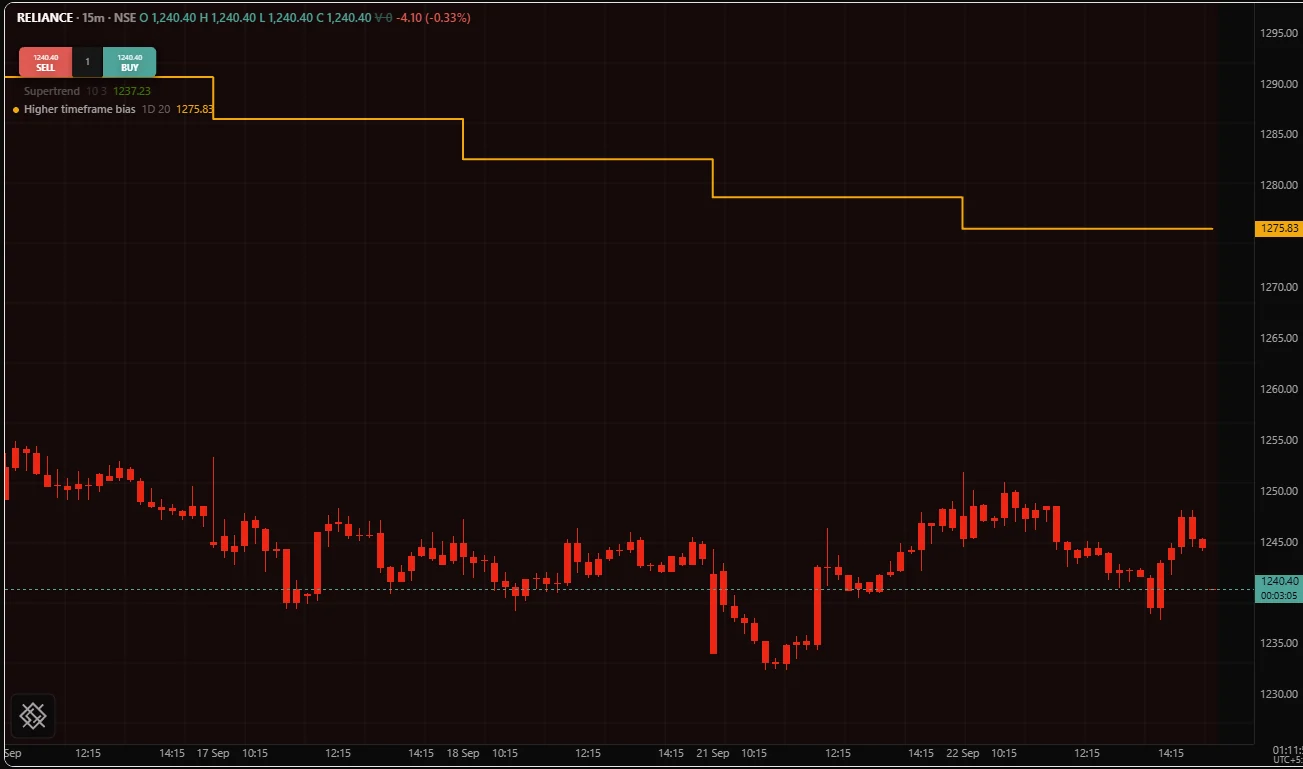
What to notice:
req.timeframe()evaluates an expression, hereema(close, biasLen), on the higher timeframe's bars. See Higher timeframes.- The mode is written out.
mode = "confirmed"is the default; writing it makes the choice visible. See Repainting. kind = "interval"makes the input a timeframe menu.- Flip markers compare
upwithup[1], throughorElse()so the first bar does not count as a flip. - The daily bars come from the chart's own bars. On the /trading chart, a read of the chart's own instrument at a longer timeframe is built from the intraday bars already loaded. A 15 minute chart loads about two months of history, enough for 20 daily closes; a 1 minute chart loads about a week, too few, and the average has no value there.
8. Dashboard
A panel fixed to a corner of the chart with the readings a discretionary trader glances at: trend, RSI and its zone, ATR as a percentage of price, where price sits in its recent range, and volume against its average. It draws no line at all.
// A panel fixed to a corner of the chart holding the readings a discretionary
// trader glances at, rather than a line drawn per bar.

version 1

study("Dashboard", overlay = true)

rsiLen  = input(14, "RSI length", min = 2, max = 200)
atrLen  = input(14, "ATR length", min = 1, max = 200)
lookback = input(20, "Range lookback", min = 2, max = 500)
corner  = input("topRight", "Corner",
                options = ["topLeft", "topRight", "bottomLeft", "bottomRight"])

// The table is declared once, before the first bar, like a plot: the chart has
// to know what it is reserving room for before any data arrives. Only the
// contents of the cells change per bar. The title comes first and is required.
panel = table("Readings", rows = 7, cols = 2, position = corner,
              textColor = silver, bgColor = fade(black, 25))

oscillator = rsi(close, rsiLen)
atrValue   = atr(atrLen)
atrPercent = atrValue / close * 100

highest20 = highest(high, lookback)
lowest20  = lowest(low, lookback)
span      = highest20 - lowest20
rangePct  = span > 0 ? (close - lowest20) / span * 100 : none

trend = ema(close, 20) > ema(close, 50)
volumeRatio = volume / sma(volume, lookback)

// One place that decides what an absent reading looks like in a cell. A blank
// cell and a zero are both wrong: the first hides that the study is still
// warming up, the second invents a number.
fn show(value, decimals) => isNone(value) ? "warming up" : text(value, decimals)

// The condition form of switch, because the arms test different things rather
// than matching one value. zone is declared before the switch: an arm cannot
// introduce a name that outlives it.
zone = "neutral"
switch
    case oscillator > 70
        zone = "overbought"
    case oscillator < 30
        zone = "oversold"
    default
        zone = "neutral"

zoneColor = oscillator > 70 ? red : oscillator < 30 ? lime : silver

// Written only on the newest bar. The panel shows one state, the current one,
// so writing it on every bar would cost thousands of writes to show the last.
// The newest bar is recomputed as each update arrives and rewrites the same
// cells.
if bar.isLast
    cell(panel, 0, 0, chart.symbol, textColor = white)
    cell(panel, 0, 1, chart.interval, textColor = white)

    cell(panel, 1, 0, "Trend")
    // Not trend ? "up" : "down" on its own: an absent condition takes the false
    // arm, so the panel would read "down" for the first fifty bars and mean it.
    cell(panel, 1, 1, isNone(trend) ? "warming up" : (trend ? "up" : "down"),
         textColor = isNone(trend) ? silver : (trend ? lime : red))

    cell(panel, 2, 0, "RSI")
    cell(panel, 2, 1, show(oscillator, 1), textColor = zoneColor)

    cell(panel, 3, 0, "Zone")
    cell(panel, 3, 1, zone, textColor = zoneColor)

    cell(panel, 4, 0, "ATR, percent of price")
    cell(panel, 4, 1, show(atrPercent, 2))

    cell(panel, 5, 0, "Position in " + text(lookback, 0) + " bar range")
    cell(panel, 5, 1, show(rangePct, 0) + " percent")

    cell(panel, 6, 0, "Volume against average")
    cell(panel, 6, 1, show(volumeRatio, 2), textColor = volumeRatio > 2 ? orange : silver)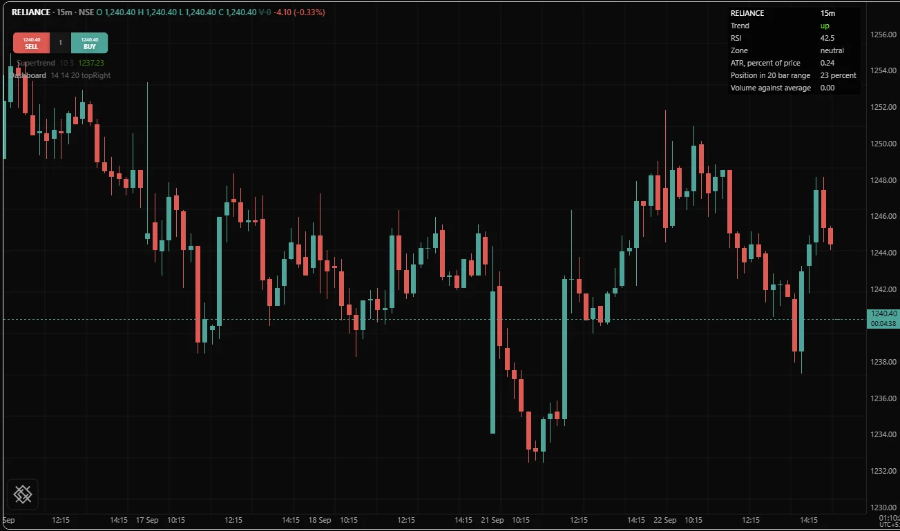
What to notice:
table()is declared at the top level, once;cell()writes into it on any bar. See Tables.bar.isLastlimits the writing to the newest bar, which is the only one the panel shows.- A user function.
fn show(value, decimals) => ...is a one-line function that turns an absent reading into the words "warming up". See User functions. switchwithout a subject runs the firstcasewhose condition is true. See Control flow.- An input as a fixed option.
position = cornertakes the corner from a menu input. A table's position is settled before the first bar, and an option settled that early accepts aninput()value directly.
9. Supply and demand zones
Supply zones drawn as boxes where price turned down, demand zones where it turned up, each extended to the right while it holds, and deleted when price closes through it or it grows too old. The whole output is geometry, so the study declares no plot.
// Supply and demand boxes drawn where price turned, extended right while they
// hold, and deleted when price closes through them or they get too old.

version 1

study("Supply and demand zones", overlay = true, precision = 2)

leftBars  = input(5,  "Pivot left bars",  min = 1, max = 50)
rightBars = input(5,  "Pivot right bars", min = 1, max = 50)
maxAge    = input(200, "Delete a zone after this many bars", min = 10, max = 5000)
maxZones  = input(12,  "Live zones per side", min = 1, max = 100)

// One array of drawing objects and four of plain numbers describing them. A
// drawing object can be changed and deleted but not read back, so the script
// remembers what it drew in order to decide later whether price has broken it.
var zones      = []
var zoneTop    = []
var zoneBottom = []
var zoneSide   = []
var zoneBar    = []

// Counted downwards, so removing element i does not renumber an element the
// loop has yet to visit. Counting upwards with a removal inside skips elements.
for i = size(zones) - 1 to 0 step -1
    top    = element(zoneTop, i)
    bottom = element(zoneBottom, i)
    side   = element(zoneSide, i)
    age    = bar.index - element(zoneBar, i)

    // A supply zone dies when price closes above it, a demand zone when price
    // closes below it. Closing through, not touching: a wick into a zone is the
    // zone working.
    broken = side > 0 ? close > top : close < bottom

    if broken or age > maxAge
        draw.delete(element(zones, i))
        remove(zones, i)
        remove(zoneTop, i)
        remove(zoneBottom, i)
        remove(zoneSide, i)
        remove(zoneBar, i)
        continue

    // Extended to this bar's own time rather than beyond it, because where the
    // next bar starts is not something the script knows.
    draw.setTo(element(zones, i), time, bottom)
    draw.setTooltip(element(zones, i), (side > 0 ? "Supply" : "Demand") +
                    ", " + text(age, 0) + " bars old")

pivotUp   = pivotHigh(high, leftBars, rightBars)
pivotDown = pivotLow(low, leftBars, rightBars)

// A zone spans the extreme of the turning bar and the far edge of its body: the
// part of the move nobody traded back through.
if not isNone(pivotUp) and size(zones) < maxZones * 2
    startTime = time[rightBars]
    zoneHigh  = high[rightBars]
    zoneLow   = max(open[rightBars], close[rightBars])
    shape = draw.box(startTime, zoneHigh, time, zoneLow,
                     color = red, fillColor = fade(red, 85), text = "Supply")
    push(zones, shape)
    push(zoneTop, zoneHigh)
    push(zoneBottom, zoneLow)
    push(zoneSide, 1)
    push(zoneBar, bar.index - rightBars)

if not isNone(pivotDown) and size(zones) < maxZones * 2
    startTime = time[rightBars]
    zoneHigh  = min(open[rightBars], close[rightBars])
    zoneLow   = low[rightBars]
    shape = draw.box(startTime, zoneHigh, time, zoneLow,
                     color = lime, fillColor = fade(lime, 85), text = "Demand")
    push(zones, shape)
    push(zoneTop, zoneHigh)
    push(zoneBottom, zoneLow)
    push(zoneSide, -1)
    push(zoneBar, bar.index - rightBars)

// This study declares no plot. Nothing it produces is one value per bar, and a
// plotted count would put a flat line across the price scale to say what the
// boxes already say.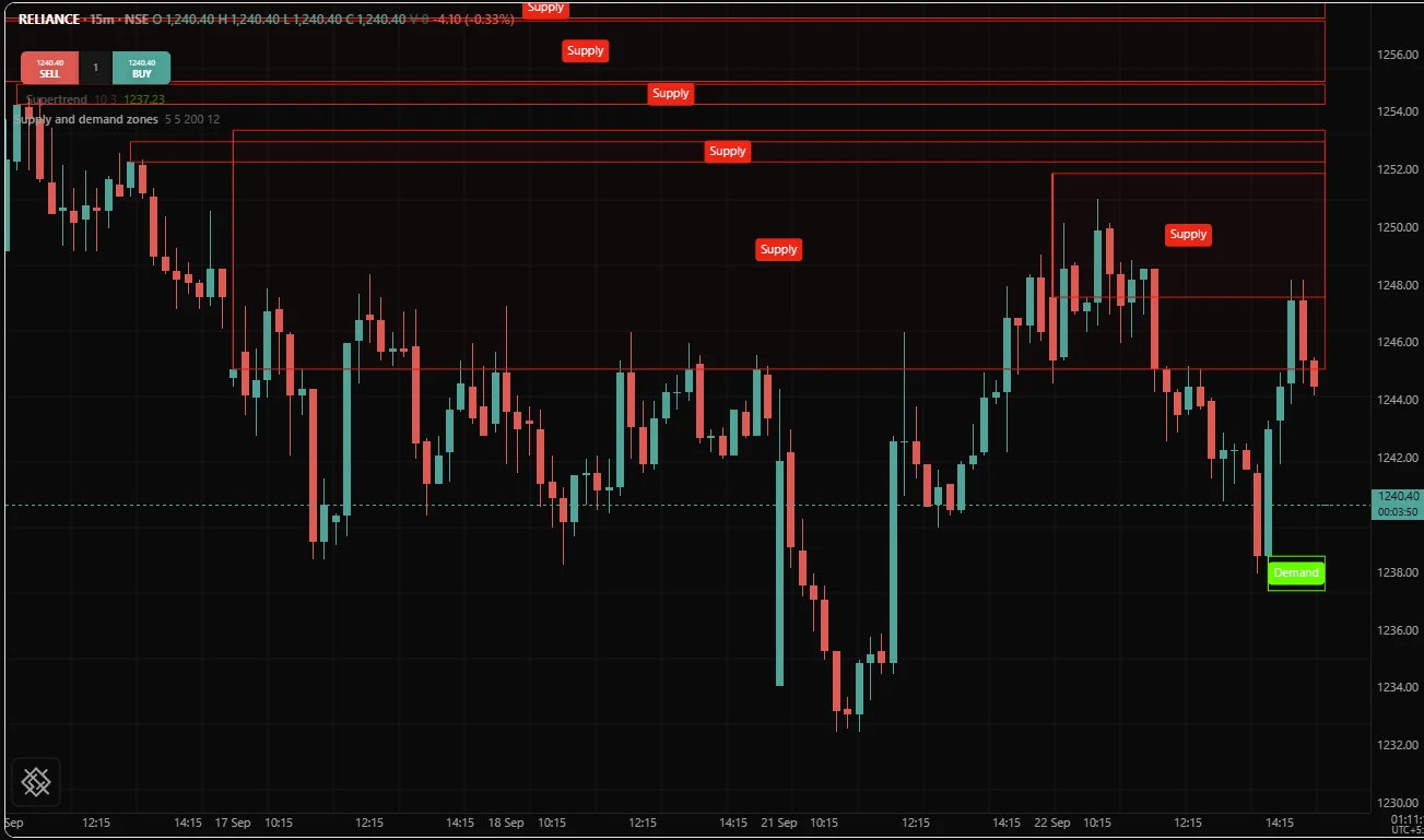
What to notice:
- Drawing objects live across bars.
draw.box()creates a box,draw.setTo()moves its right edge, anddraw.delete()removes it. See Lines and boxes. - Arrays in
var.var zones = []is created once and kept;push(),remove(),element()andsize()manage it. See Collections. - A descending loop.
step -1walks the list from the end, so a removal never skips the next element.continuemoves on to the next zone. - No plot is fine. A study whose whole output is drawings needs no
plot.
10. EMA cross, bracketed
The crossing from script 1, traded: a long entry on the upward cross, a stop and a target fixed at entry from the ATR, a size chosen so every trade risks the same amount, and an exit on the downward cross. It also declares its capital and costs.
// The same crossing as the first example, traded: a stop and a target fixed at
// entry, and a size chosen so that the stop costs the same on every trade.

version 1

strategy("EMA cross, bracketed", overlay = true, precision = 2,
         capital = 500000, qtyType = "units", qty = 1,
         product = "intraday", pyramiding = 1,
         fillOn = "nextOpen", slippage = 1,
         commissionType = "perTrade", commission = 20)

fastLen    = input(9,    "Fast length", min = 1, max = 500)
slowLen    = input(21,   "Slow length", min = 1, max = 500)
atrLen     = input(14,   "ATR length",  min = 1, max = 200)
stopMult   = input(2.0,  "Stop, in ATR",   min = 0.2, max = 20)
targetMult = input(3.0,  "Target, in ATR", min = 0.2, max = 40)
riskAmount = input(5000, "Amount risked per trade", min = 1)

fast = ema(close, fastLen)
slow = ema(close, slowLen)
atrValue = atr(atrLen)

stopDistance   = stopMult * atrValue
targetDistance = targetMult * atrValue

// Size from the distance to the stop, so a wide stop buys fewer units and every
// trade risks the same amount of money.

// chart.lotSize is absent, not 1, when the host has not said what a lot is, and
// absence passes through max as it does through arithmetic. So the fallback
// goes inside: without orElse every size would be absent and the strategy would
// never place an order.
lotUnits  = max(orElse(chart.lotSize, 1), 1)
rawUnits  = stopDistance > 0 ? riskAmount / stopDistance : none
orderQty  = isNone(rawUnits) ? none : floor(rawUnits / lotUnits) * lotUnits

var entryStop   = none
var entryTarget = none

flat    = pos.size == 0
canSize = not isNone(orderQty) and orderQty > 0

if crossUp(fast, slow) and flat and canSize
    // The levels come from this bar's close, and the order fills at the next
    // bar's open, which is the default and the honest one. The report shows the
    // slippage between the two rather than hiding it.
    //
    // exit() takes absolute prices, and both levels go in one call, never two,
    // so a gap through both cannot fill them as separate orders.
    entryStop   = close - stopDistance
    entryTarget = close + targetDistance
    buy(qty = orderQty, tag = "entry")
    exit(tag = "entry", stop = entryStop, limit = entryTarget)

if crossDown(fast, slow) and pos.size > 0
    entryStop   = none
    entryTarget = none
    close()

plot(fast, "Fast", aqua, width = 2)
plot(slow, "Slow", orange, width = 2)

// The stop as sent, not as it would be recomputed now. Plotting the distance
// from the current close would draw a line that trails the price and was never
// an order.
plot(pos.size > 0 ? entryStop : none,   "Stop",   red,  style = "step")
plot(pos.size > 0 ? entryTarget : none, "Target", lime, style = "step")
plot(pos.size > 0 ? pos.avgPrice : none, "Entry", fade(silver, 40), style = "step")
What to notice:
- A strategy is a study with orders. The same crossing as script 1, with
buy(),exit()andclose()added and the declaration changed. - Risk-based sizing by hand. The size is the money at risk divided by the stop distance, rounded down to whole lots with
floor().chart.lotSizeis absent when the host states no lot size, soorElse()supplies 1. - Levels held in
varare the levels actually sent, so the plotted stop is the stop the trade was opened with. pos.sizeandpos.avgPriceread the position from fills.
11. Opening range breakout
The opening range of script 5, traded once per session: long on a close above the range, short on a close below it, the far side of the range as the stop, a target at a multiple of the range width, and a hard exit five hours after the open. Sized in lots, for an index future on NFO or a commodity future on MCX.
// The opening range of the fifth example, traded once per session, with the
// other side of the range as the stop and a hard exit by the clock.

version 1

strategy("Opening range breakout", overlay = true, precision = 2,
         capital = 500000, qtyType = "lots", qty = 1,
         product = "intraday", pyramiding = 1, closeOnSessionEnd = true,
         fillOn = "nextOpen", slippage = 1,
         commissionType = "perTrade", commission = 20)

rangeMinutes = input(15,  "Opening range, in minutes", min = 1, max = 240)
holdMinutes  = input(300, "Flat this many minutes after the open", min = 5, max = 1440)
targetMult   = input(2.0, "Target, in range widths", min = 0.2, max = 10)
lots         = input(1,   "Lots", min = 1, max = 100)

var openTime  = none
var rangeHigh = none
var rangeLow  = none
var traded    = false

if session.isFirstBar
    openTime  = time
    rangeHigh = high
    rangeLow  = low
    traded    = false

elapsed = isNone(openTime) ? none : time - openTime
forming = not isNone(elapsed) and elapsed < rangeMinutes * 60000

if forming and not session.isFirstBar
    rangeHigh = max(rangeHigh, high)
    rangeLow  = min(rangeLow, low)

rangeWidth = isNone(rangeHigh) ? none : rangeHigh - rangeLow

// One entry per session, and only after the range has finished forming. traded
// is set at the entry rather than cleared at the exit, so a trade stopped out
// at ten past the open does not re-enter at quarter past.
ready = not forming and not traded and pos.size == 0
ok    = not isNone(rangeWidth) and rangeWidth > 0

if ready and ok and close > rangeHigh
    traded = true
    buy(qty = lots, tag = "entry")
    // The far side of the range is the stop, because that is the level that
    // says the breakout was wrong. A multiple of volatility would be a second
    // opinion about a level the market has already drawn.
    exit(tag = "entry", stop = rangeLow, limit = rangeHigh + rangeWidth * targetMult)

if ready and ok and close < rangeLow
    traded = true
    sell(qty = lots, tag = "entry")
    exit(tag = "entry", stop = rangeHigh, limit = rangeLow - rangeWidth * targetMult)

// The clock exit is neither a stop nor a target: it is the admission that a
// position that has not worked in five hours is not going to. closeOnSessionEnd
// is declared as well, for hosts that state session hours; /trading states
// none in this release, so there it has no effect.
if pos.size != 0 and not isNone(elapsed) and elapsed >= holdMinutes * 60000
    close()

highPlot = plot(rangeHigh, "Range high", aqua,   width = 2, style = "step")
lowPlot  = plot(rangeLow,  "Range low",  orange, width = 2, style = "step")
fill(highPlot, lowPlot, fade(aqua, 93))
background(forming ? fade(silver, 92) : none)
What to notice:
- Both directions.
sell()opens a short on the downside break, and the sameexit()call protects either side. qtyType = "lots"counts the order size in lots, converted to units through the instrument's lot size.- One trade per session, held in
var traded, reset onsession.isFirstBar. - A time exit.
elapsed >= holdMinutes * 60000flattens withclose()five hours after the open, before the NSE close at 15:30 IST.
12. Short premium, combined stop
Two option legs sold together and managed as one position: one stop, one target and one clock exit, all measured on the sum of the two prices. The chart carries one leg, for example the NIFTY call; the script reads the other with req.symbol() and raises an alert for it, because a strategy trades the instrument on its chart.
// Two option legs sold together and managed as one position: one stop, one
// target, one clock exit, all measured on the sum of the two prices rather than
// on either leg.

version 1

strategy("Short premium, combined stop", precision = 2,
         capital = 500000, qtyType = "lots", qty = 1,
         product = "intraday", pyramiding = 1, closeOnSessionEnd = true,
         fillOn = "nextOpen", slippage = 1,
         commissionType = "perTrade", commission = 20)

// A plain text input: type the other leg's trading symbol. An instrument picker
// input is planned, and until it exists the leg is typed in.
otherLeg    = input("", "The other leg's symbol")
lots        = input(1,  "Lots per leg", min = 1, max = 100)
tradeDay    = input(4,  "Weekday to trade, 1 is Monday", min = 1, max = 7)
entryMinute = input(20, "Enter this many minutes after the open", min = 0, max = 1440)
exitMinute  = input(330, "Flat this many minutes after the open", min = 1, max = 1440)
stopPct     = input(30, "Stop, in percent of the entry premium", min = 1, max = 500)
targetPct   = input(50, "Target, in percent of the entry premium", min = 1, max = 99)

// The chart carries one leg and the script reads the other. A leg the chart
// does not show has no bars a backtest could fill against, so this script
// trades the chart's leg and routes the other through the alerts below.
otherPrice = req.symbol(otherLeg, chart.interval, close, exchange = chart.exchange)

// The position is the sum, so the sum is what is managed. Stopping each leg
// separately is the classic way to take two losses on a day the legs were
// hedging each other.
premium = close + otherPrice

var openTime     = none
var entryPremium = none
var doneToday    = false

if session.isFirstBar
    openTime  = time
    doneToday = false

// Cleared before the entry below can set a fresh one, so a position closed at
// the session end does not leave its entry premium behind for the next day.
// Written the other way round, it would wipe the level on the entry bar itself,
// because the position is still flat until the fill.
if pos.isFlat
    entryPremium = none

elapsed = isNone(openTime) ? none : time - openTime

// A day of the week rather than a list of dates, because the day this strategy
// wants recurs every week and a list of dates goes stale.
rightDay   = date.dayOfWeek(time) == tradeDay
priced     = not isNone(premium)
afterEntry = not isNone(elapsed) and elapsed >= entryMinute * 60000
afterExit  = not isNone(elapsed) and elapsed >= exitMinute * 60000

if rightDay and priced and afterEntry and pos.isFlat and not doneToday
    sell(qty = lots, tag = "premium")
    entryPremium = premium
    doneToday    = true
    alert("SELL " + text(lots, 0) + " lots of " + otherLeg, id = "other-leg-entry")

// Positive when the seller is losing, which is the direction the stop cares
// about. Absence does the guarding: entryPremium is absent while flat and
// premium is absent whenever either leg has no bar, so movePct is absent and no
// test below is true.
movePct = (premium - entryPremium) / entryPremium * 100

hit     = not isNone(movePct) and movePct >= stopPct
banked  = not isNone(movePct) and movePct <= -targetPct
timeOut = afterExit

// One close, with the reason attached, rather than three blocks that could each
// send one on the same bar. The position stays short until the fill on the next
// bar's open, so three blocks whose conditions were all true would send three
// closing orders against one short position.
if pos.isShort and (hit or banked or timeOut)
    close()
    alert("BUY " + text(lots, 0) + " lots of " + otherLeg, id = "other-leg-exit")
    signal(hit ? "STOP" : (banked ? "TARGET" : "TIME"))

// No ternary on these: entryPremium is absent while flat, absence passes through
// the arithmetic, and a plot given an absent value draws a gap, not a zero.
plot(premium, "Combined premium", orange, width = 2)
plot(entryPremium, "Entry premium", fade(silver, 40), style = "step")
plot(entryPremium * (1 + stopPct / 100), "Stop", red, style = "step")
plot(entryPremium * (1 - targetPct / 100), "Target", lime, style = "step")
What to notice:
- Managed on the sum. The stop and target are percentages of the combined entry premium, not of either leg.
- A weekly schedule.
date.dayOfWeek()picks the weekday, for example the day before a weekly expiry. - Absence as a guard. While flat,
entryPremiumisnone, somovePctisnoneand none of the exit tests can be true. - One exit with a reason. A single
close()carries the reason in itssignal()marker, so the position can never be closed three times over. - The second leg is an alert. The strategy trades the chart's leg; the other leg's orders go out as
alert()messages with their own ids. On /trading this script does not run today, as the note below explains.
Showcase scripts
Three more studies, written to look their best on a chart as well as to teach. Each file below is the exact script that drew the screenshot under it, so what you paste is what you see. All three are studies: they draw on the /trading chart as described and place no orders.
HalfTrend
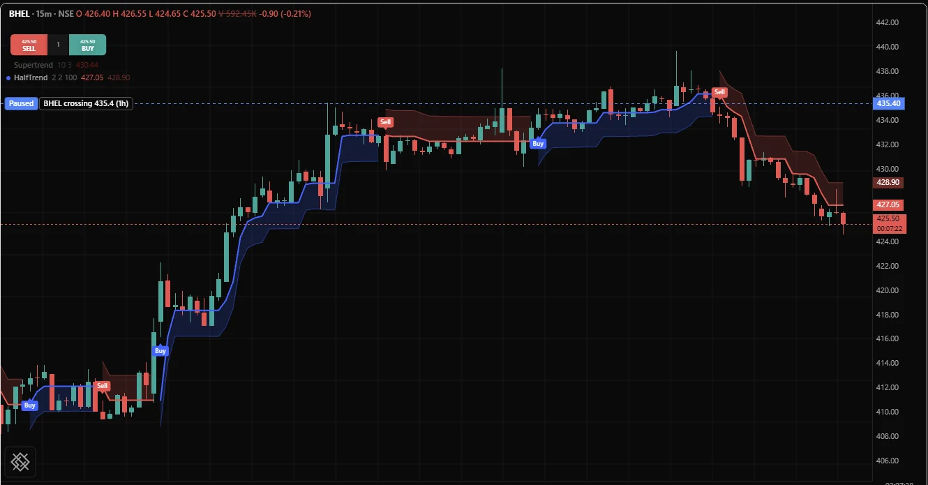
A trend level that holds flat through noise and turns only when the other side of the recent range gives way. While the trend is up, the study keeps the highest value the low of that range has reached since the turn, and it turns down when the average high of the last few bars falls below it and the bar closes below the previous bar's low. A downtrend is the mirror image. The level is blue while the trend is up and red while it is down, a shaded channel rides beside it, and every flip is labelled. Amplitude is the number of bars in the range it watches, and the channel sits a multiple of half the average true range (atr()) away from the level.
// HalfTrend: a trend level that holds flat through noise and turns only when
// the other side of the range gives way. Blue while the trend is up, red while
// it is down, with a shaded channel and a label on every flip.
version 1

study("HalfTrend", overlay = true, precision = 2)

amplitude = input(2, "Amplitude", min = 1, max = 100)
channelDev = input(2, "Channel deviation", min = 0, max = 20)
atrLen = input(100, "ATR length", min = 1, max = 500)

half = atr(atrLen) / 2
dev = channelDev * half
rollHigh = highest(high, amplitude)
rollLow = lowest(low, amplitude)
meanHigh = sma(high, amplitude)
meanLow = sma(low, amplitude)
prevHigh = bar.isFirst ? high : high[1]
prevLow = bar.isFirst ? low : low[1]

// trend is 0 while up and 1 while down; armed is the flip being watched for.
var trend = 0
var armed = 0
var maxLow = low
var minHigh = high
var upLevel = low
var downLevel = high

wasTrend = bar.isFirst ? -1 : trend

if armed == 1
    maxLow = max(orElse(rollLow, maxLow), maxLow)
    if not isNone(meanHigh) and meanHigh < maxLow and close < prevLow
        trend = 1
        armed = 0
        minHigh = orElse(rollHigh, high)
else
    minHigh = min(orElse(rollHigh, minHigh), minHigh)
    if not isNone(meanLow) and meanLow > minHigh and close > prevHigh
        trend = 0
        armed = 1
        maxLow = orElse(rollLow, low)

flipUp = trend == 0 and wasTrend == 1
flipDown = trend == 1 and wasTrend == 0

// On a flip the new level starts where the other side ended, so it steps.
if trend == 0
    upLevel = flipUp ? downLevel : wasTrend == -1 ? maxLow : max(maxLow, upLevel)
else
    downLevel = flipDown ? upLevel : wasTrend == -1 ? minHigh : min(minHigh, downLevel)

ht = trend == 0 ? upLevel : downLevel

upLine = plot(trend == 0 ? ht : none, "Up trend", #2962ff, width = 2)
downLine = plot(trend == 1 ? ht : none, "Down trend", #ef5350, width = 2)
upEdge = plot(trend == 0 ? ht - dev : none, "Channel low", fade(#2962ff, 55), width = 1)
downEdge = plot(trend == 1 ? ht + dev : none, "Channel high", fade(#ef5350, 55), width = 1)
fill(upLine, upEdge, fade(#2962ff, 82))
fill(downLine, downEdge, fade(#ef5350, 82))

if flipUp
    signal("Buy", #2962ff, at = "below", shape = "label")

if flipDown
    signal("Sell", #ef5350, at = "above", shape = "label")
On a BHEL 15 minute NSE chart with the default settings:
What it shows:
- State carried across bars.
trend,armed,maxLow,minHigh,upLevelanddownLevelare declared withvar, so each is set once, on the first bar, and then starts every bar from the value the previous bar left.wasTrendreadstrendabove the lines that reassign it, so it holds the previous bar's trend, and-1on the first bar, so nothing there counts as a flip. See Persistence. - Two plots, so the line can change colour.
Up trendhas a value only while the trend is up andDown trendonly while it is down; each isnoneon the other side. A flip is a clean step from one line to the other, never a diagonal drawn through the candles. - Fills to a channel edge. Each level has a faint edge plot
devaway from it, below the up level and above the down level, andfill()shades between the level and its edge. The fill colours are written in the call withfade(), so the chart draws them as given. - A label on a flip.
flipUpandflipDowncompare this bar's trend withwasTrend, andsignal()withshape = "label"puts a Buy plate on the bar that turned up (at = "below") and a Sell plate on the bar that turned down (at = "above"). - The start of the chart, handled.
orElse()supplies a starting value whilehighest()andlowest()have none yet, and theisNone()tests make each flip test wait until the averages it compares have values.
Bollinger Bands
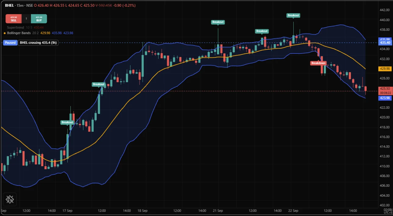
A 20 bar simple average with bands two standard deviations either side of it, the space between the bands shaded, and a label where price closes outside a band. Wide bands mean a volatile market, narrow ones a quiet one.
// Bollinger Bands: a 20 bar mean with bands two standard deviations either
// side, the space between them shaded, and a label where price closes
// outside a band.
version 1

study("Bollinger Bands", overlay = true, precision = 2)

len = input(20, "Length", min = 1, max = 500)
mult = input(2, "Deviations", min = 0.5, max = 5)

bb = bollinger(close, len, mult)
basis = bb[0]
upper = bb[1]
lower = bb[2]

plot(basis, "Basis", orange, width = 2)
upperPlot = plot(upper, "Upper", #2962ff, width = 1.5)
lowerPlot = plot(lower, "Lower", #2962ff, width = 1.5)
fill(upperPlot, lowerPlot, fade(#2962ff, 88))

if crossUp(close, upper)
    signal("Breakout", #26a69a, at = "above", shape = "label")

if crossDown(close, lower)
    signal("Breakdown", #ef5350, at = "below", shape = "label")
On a BHEL 15 minute NSE chart with the default settings:
What it shows:
- A function with several outputs.
bollinger()returns the basis, the upper band and the lower band in one array, from one call and one piece of state. The script names each one,basis = bb[0]and so on, so the rest of the file reads as words rather than positions. See Plotting a function with several outputs. - A fill between two plots. The two bands are plotted into named handles,
upperPlotandlowerPlot, andfill()shades between them. The basis needs no handle, because nothing fills to it. - Signals on a band cross.
crossUp()of the close over the upper band marks a Breakout, andcrossDown()of the close under the lower band marks a Breakdown. Each is written in anifcondition at the top level, so it runs on every bar and never misses a crossing. - Inputs with limits.
minandmaxon eachinput()keep the settings dialog to lengths and widths that make sense.
EMA cross in colour
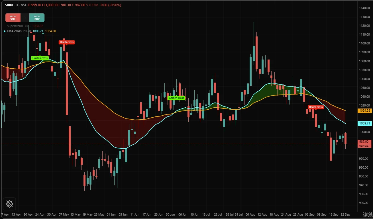
Script 1 dressed for the chart: a 20 and a 50 bar exponential average, the band between them green while the fast average leads and red while the slow one does, and a labelled marker on every crossover. The labels use the traditional names: a golden cross for an upward cross and a death cross for a downward one.
// EMA cross: a fast and a slow exponential average, the band between them
// shaded by trend, and a labelled marker on every crossover.
version 1

study("EMA cross", overlay = true, precision = 2)

fastLen = input(20, "Fast length", min = 1, max = 500)
slowLen = input(50, "Slow length", min = 1, max = 500)

fast = ema(close, fastLen)
slow = ema(close, slowLen)

fastPlot = plot(fast, "Fast EMA", aqua, width = 2)
slowPlot = plot(slow, "Slow EMA", orange, width = 2)

// Green while the fast average is above the slow one, red while below.
fill(fastPlot, slowPlot, colorUp = fade(lime, 80), colorDown = fade(red, 80))

if crossUp(fast, slow)
    signal("Golden cross", lime, at = "below", shape = "label")

if crossDown(fast, slow)
    signal("Death cross", red, at = "above", shape = "label")
On a daily SBIN chart:
What it shows:
- One fill, two colours.
fill()withcolorUpandcolorDowncolours the band by which plot is on top.colorUpapplies where the first plot named,fastPlot, is at or above the second, so green means the fast average leads. See Fills. - Labelled crossovers. Each
signal()states its text, its colour, its side of the bar and its shape, so a Golden cross is a lime plate below the bar and a Death cross a red plate above it. - Transparency in the colours.
fade(lime, 80)andfade(red, 80)carry the band's transparency andopacityis left alone, which is how Fills recommends shading a band with two colours.
Related. Quickstart, Your first strategy, Visuals overview, Strategies overview, Style guide, Troubleshooting