
Technical analysis
Every indicator function in OpenScript, grouped by purpose: moving averages, trend, oscillators and momentum, volatility and bands, volume, and swings. Each entry says what the indicator measures, how to read it and gives a script you can paste.
On this page
This page is the reference for every indicator built into OpenScript, also called OpenAlgo Script: sixty-eight functions from the simple moving average to the Ichimoku cloud. Fifty-five of them work in version 0.5.0; the other thirteen are named in the language and marked Planned, so you can see what is coming. Each entry tells you what the indicator measures, how traders read it, the exact arithmetic where it matters, and the first bar on which it has a value. Every example is a complete script: paste it into the Scripts panel of the /trading page, save it, and press Apply to chart.
You need this page whenever a study or strategy reads price through an indicator. Indicators are where most scripts start, and most surprises in a new script (a line that starts late, a crossing that never fires, a band that is missing on the left of the chart) come from the details written here.
How to read an entry
Each entry opens with a short description. Below it the compiler fills in the signature, a table of parameters with their types and defaults, the return type and the first value: the first bar on which the call can return a number, counting the oldest bar loaded on the chart as bar 0. Below those facts you find a working example, remarks and links to related entries.
A few rules hold for every function on the page.
- Warmup is exact. Before its first value a call returns
none, the absent value, and a plot shows a gap there rather than a zero. After it, the call has a value on every bar whose inputs are present, except where the arithmetic would divide by zero (a window with no range, for example); the remarks of each entry name those cases. Warmups add up when you feed one indicator into another:sma(ema(close, 10), 10)has its first value on bar 18, because the inner average starts on bar 9 and the outer one then needs ten values. See Warmup and Absent values. - Absence spreads through a window. If any bar inside a window is absent, that bar's result is absent. Only
sumSkip(),avgSkip()andcountPresent()skip absent values, and they say so in their names. - A length is a whole number of 1 or more. Any other value, such as
0or2.5, stops the script on the first bar that uses it with run-time error OS4003. Take a length frominput()so the user can change it, and keep it fixed while the script runs: if a computed length changes between bars, a window function such assma()starts its window again and is absent until the new window fills. - Every indicator call keeps its own state. An
emaremembers its running value from one bar to the next, which is why almost every entry carries a Keeps state badge. The state belongs to the place the call is written, so each call in your file is a separate indicator. Assign an indicator to a name once and reuse the name rather than writing the same call twice. - Compute indicators at the top level, on every bar. A call that keeps state only advances on the bars where it actually runs. Inside an
ifblock, in the side of acondition ? a : bchoice that is not taken, or on the right of anandororthat has already decided its answer, it skips bars and draws a different line. The compiler warns about all three with OS8001:
trend = 0.0
if close > open
    trend = ema(close, 20)
The fix is to compute first and decide afterwards:
version 1
study("Compute first, decide after", overlay = true)

avg20 = ema(close, 20)
plot(close > open ? avg20 : none, "EMA 20 on up bars", aqua)Functions that return several values
Some indicators produce more than one line: MACD has a line, a signal and a histogram. These functions return an array<number> holding this bar's values in a fixed order. Read each value by its position with [0], [1] and so on.
version 1
study("MACD, three lines", precision = 2)

m = macd(close, 12, 26, 9)

plot(m[0], "MACD", aqua)
plot(m[1], "Signal", orange)
plot(m[2], "Histogram", gray, style = "histogram")
The array always has the same length, even during warmup. Each position carries its own warmup and holds none until it is reached, so m[1] is never an out-of-range error on an early bar.
| Function | [0] | [1] | [2] | [3] | [4] |
|---|---|---|---|---|---|
macd() | MACD line | Signal | Histogram | ||
ppo() | PPO line | Signal | Histogram | ||
stoch() | %K | %D | |||
stochRsi() | %K | %D | |||
bollinger() | Basis | Upper | Lower | ||
keltner() | Basis | Upper | Lower | ||
donchian() | Upper | Middle | Lower | ||
supertrend() | Line | Direction | |||
psar() | Stop | Direction | |||
adx() | ADX | +DI | -DI | ||
aroon() | Up | Down | |||
ichimoku() | Conversion | Base | Span A | Span B | Lagging |
In m[1] the brackets pick an element of the array, not a past bar. To read an element's value on an earlier bar, give it a name first; a top-level name has history, and [1] on it means one bar ago.
version 1
study("Signal line rising", precision = 2)

m   = macd(close)
sig = m[1]

plot(sig, "Signal", sig > sig[1] ? lime : red, width = 2)
Writing both steps on one expression is an error, because an element has no history of its own:
st = supertrend(3, 10)
flipped = st[1] != st[1][1]
Name the element first, as sig = m[1] does above, and read its history from the name.
Choosing a moving average
Every average smooths price and every average lags it. They differ in how they trade smoothness for speed.
| You want | Use | Trade-off |
|---|---|---|
| The plain average everyone means by "the 200 day" | sma() | Equal weights; reacts slowly and drops old bars abruptly |
| A faster average that never fully forgets | ema() | Weight 2 / (len + 1) on the newest bar |
| The smoothing inside RSI, ATR and ADX | rma() | Weight 1 / len; slower than an ema of the same length |
| Recent bars to count more, in a straight line | wma() | Newest bar weighted len, oldest weighted 1 |
| Much less lag at the same length | hma() | Can overshoot at turns; longer warmup |
An ema with its lag partly removed | dema(), tema() | Longer warmup; can overshoot |
| Heavily traded bars to count more | vwma() | Needs volume |
| A tunable balance of lag and smoothness | alma() | Two extra settings to choose |
| The end point of a fitted trend line | linreg() | Follows straight trends closely; jumps at turns |
| A light four-bar smoothing with no length | swma() | Fixed at four bars |
| Let the user choose from the settings dialog | ma() | Only the six common types |
Moving averages
sma()
The simple moving average: the arithmetic mean of the last len values of src, every bar weighted equally. It is the baseline average and the one traders mean by "the 50 day" and "the 200 day" on a daily chart.
sma(src: series number, len: number) -> series number| Parameter | Type | Default | Notes |
|---|---|---|---|
src | series number | required | |
len | number | required |
- Returns
series number- First value
- bar
len - 1
version 1
study("50 and 200 day averages", overlay = true)

sma50  = sma(close, 50)
sma200 = sma(close, 200)

plot(sma50, "SMA 50", aqua)
plot(sma200, "SMA 200", orange, width = 2)

if crossUp(sma50, sma200)
    signal("GOLDEN CROSS", color = lime, at = "below", shape = "triangleUp")
if crossDown(sma50, sma200)
    signal("DEATH CROSS", color = red, at = "above", shape = "triangleDown")
Remarks. A 200 bar average has no value until bar 199, which on a daily NSE chart is roughly ten months of sessions, so load enough history before you judge the line. The sum is taken afresh over the window on every bar, oldest value first, and divided once by len. The cost per bar grows with len but not with the length of the chart. An absent value anywhere in the window makes that bar's average absent.
ema()
The exponential moving average gives the newest value a weight of 2 / (len + 1) and the running average the rest, so recent bars count more and old bars fade away without ever dropping out abruptly. It reacts to a new move sooner than sma() of the same length, which makes it the usual choice for crossover systems.
ema(src: series number, len: number) -> series number| Parameter | Type | Default | Notes |
|---|---|---|---|
src | series number | required | |
len | number | required |
- Returns
series number- First value
- bar
len - 1
version 1
study("EMA 9 and 21", overlay = true)

fastLen = input(9, "Fast", min = 1, max = 200)
slowLen = input(21, "Slow", min = 2, max = 400)

fast = ema(close, fastLen)
slow = ema(close, slowLen)

fastPlot = plot(fast, "EMA fast", aqua, width = 2)
slowPlot = plot(slow, "EMA slow", orange, width = 2)
fill(fastPlot, slowPlot, colorUp = fade(lime, 88), colorDown = fade(red, 88))

if crossUp(fast, slow)
    signal("BUY", color = lime, at = "below", shape = "arrowUp")
if crossDown(fast, slow)
    signal("SELL", color = red, at = "above", shape = "arrowDown")
The picture shows a 20 and 50 bar variant of this study on a daily SBIN chart, with the band shaded the same way and each crossing labelled Golden cross or Death cross in place of an arrow:
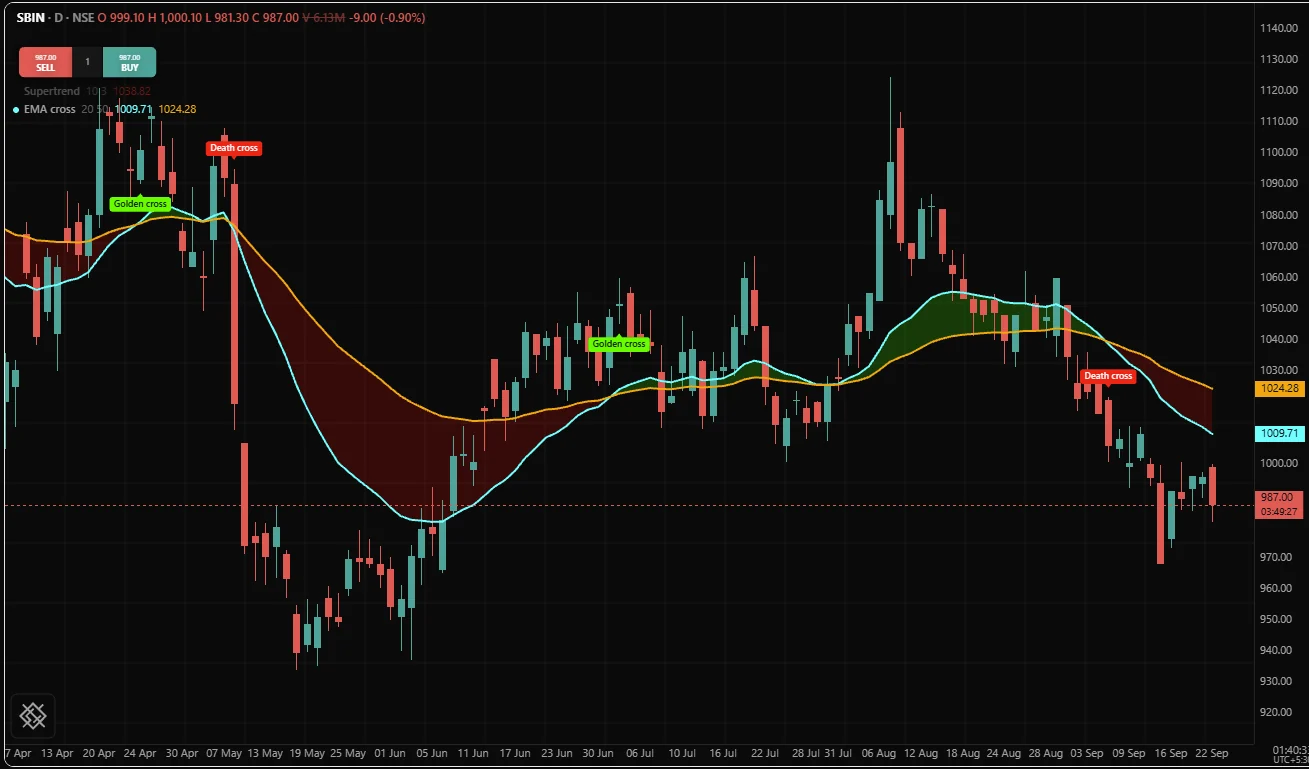
Remarks. The average is seeded on bar len - 1 with the simple average of the first len values, and is absent before that. It does not start from the first close and drift into shape, so the line you see is correct from its first point. Each later bar computes value * weight + previous * (1 - weight). With len of 9 the newest close carries 20 percent of the weight. If the source is absent on a bar after the seed, that bar's result is absent and the running value is held, so the next present bar carries on where the last one left off.
wma()
The weighted moving average weights the last len values in a straight line: the newest value counts len times, the one before it len - 1 times, down to 1 for the oldest. At the same length it turns sooner than both sma() and ema(), and it forgets a bar completely once the bar leaves the window.
wma(src: series number, len: number) -> series number| Parameter | Type | Default | Notes |
|---|---|---|---|
src | series number | required | |
len | number | required |
- Returns
series number- First value
- bar
len - 1
version 1
study("WMA against SMA", overlay = true)

len = input(20, "Length", min = 1, max = 500)

plot(wma(close, len), "WMA", lime, width = 2)
plot(sma(close, len), "SMA", fade(silver, 30))
Remarks. The weighted sum is divided once by len * (len + 1) / 2, the total of the weights. With len of 20 the newest bar carries 20 of 210 parts, just under 10 percent. hma() is built from three of these averages.
rma()
The running moving average, often called Wilder's smoothing: an exponential average whose newest value gets a weight of 1 / len. It is the smoothing inside rsi(), atr() and adx(), and you reach for it when you rebuild or adapt one of those indicators yourself.
rma(src: series number, len: number) -> series number| Parameter | Type | Default | Notes |
|---|---|---|---|
src | series number | required | |
len | number | required |
- Returns
series number- First value
- bar
len - 1
version 1
study("RSI built from rma", precision = 2, range = [0, 100])

len = input(14, "Length", min = 1, max = 200)

delta = change(close)
gain  = max(delta, 0)
loss  = max(-delta, 0)

avgGain = rma(gain, len)
avgLoss = rma(loss, len)
manual  = avgLoss == 0 ? 100 : 100 - 100 / (1 + avgGain / avgLoss)

plot(manual, "RSI by hand", purple, width = 2)
plot(rsi(close, len), "rsi()", fade(orange, 40))
The two lines in this example lie on top of each other, because this is how rsi() is defined.
Remarks. Seeded like ema(): on bar len - 1, with the simple average of the first len values. Each later bar computes (previous * (len - 1) + value) / len. A weight of 1 / len is the same decay as an ema of length 2 * len - 1, so rma(x, 14) moves about as slowly as ema(x, 27). Keep that in mind when you compare the two.
hma()
The Hull moving average combines weighted averages so that most of the lag cancels out: it follows price closely while staying smooth. Traders often colour it by its slope and treat a change of slope as a change of trend.
hma(src: series number, len: number) -> series number| Parameter | Type | Default | Notes |
|---|---|---|---|
src | series number | required | |
len | number | required |
- Returns
series number- First value
- bar
len + round(sqrt(len)) - 2
version 1
study("Hull average", overlay = true)

len = input(55, "Length", min = 2, max = 500)
h = hma(close, len)

plot(h, "HMA", h > h[1] ? lime : red, width = 2)
Remarks. The recipe is wma(2 * wma(src, half) - wma(src, len), round(sqrt(len))), where half is floor(len / 2) held at a minimum of 1. The first value arrives on bar len + round(sqrt(len)) - 2, bar 60 for a length of 55. Because it removes lag by extrapolating, it can overshoot price at sharp turns.
dema()
The double exponential moving average subtracts an average's own lag once: 2 * ema - ema(ema). It hugs price more closely than ema() of the same length.
dema(src: series number, len: number) -> series number| Parameter | Type | Default | Notes |
|---|---|---|---|
src | series number | required | |
len | number | required |
- Returns
series number- First value
- bar
2 * len - 2
version 1
study("DEMA against EMA", overlay = true)

len = input(20, "Length", min = 1, max = 300)

plot(ema(close, len), "EMA", fade(silver, 30))
plot(dema(close, len), "DEMA", aqua, width = 2)
Remarks. The second average is fed the first one's output, absent bars included, so it seeds on the first len values the first one produced. That gives the first value on bar 2 * len - 2, bar 38 for a length of 20.
tema()
The triple exponential moving average applies the same lag correction twice: 3 * e1 - 3 * e2 + e3, where e1 is the ema of the source, e2 the ema of e1 and e3 the ema of e2. It is the fastest of the exponential family and the most prone to overshoot.
tema(src: series number, len: number) -> series number| Parameter | Type | Default | Notes |
|---|---|---|---|
src | series number | required | |
len | number | required |
- Returns
series number- First value
- bar
3 * len - 3
version 1
study("Triple EMA trend", overlay = true)

len = input(20, "Length", min = 1, max = 200)
t = tema(close, len)

plot(t, "TEMA", t > t[1] ? teal : maroon, width = 2)
Remarks. Three chained averages need three warmups, so the first value is on bar 3 * len - 3, bar 57 for a length of 20. trix() measures the rate of change of the same triple smoothing.
vwma()
The volume weighted moving average weights each value by the volume traded on its bar, so a heavily traded bar pulls the average more than a quiet one. When it sits above sma() of the same length, the higher closes came on heavier volume.
vwma(src: series number, len: number) -> series number| Parameter | Type | Default | Notes |
|---|---|---|---|
src | series number | required | |
len | number | required |
- Returns
series number- First value
- bar
len - 1
version 1
study("VWMA against SMA", overlay = true)

len = input(20, "Length", min = 1, max = 500)

v = vwma(close, len)
s = sma(close, len)

vPlot = plot(v, "VWMA", orange, width = 2)
sPlot = plot(s, "SMA", fade(silver, 30))
fill(vPlot, sPlot, colorUp = fade(lime, 85), colorDown = fade(red, 85))
Remarks. It is the window sum of src * volume divided by the window sum of volume. It is absent where any bar in the window has no volume, and where the volume in the window adds up to zero. An index itself, such as NIFTY 50, trades no volume, so there is nothing to weight by on an index chart: chart the index future on NFO instead.
swma()
The symmetric weighted moving average is a fixed four-bar smoothing with weights 1, 2, 2 and 1. It has no length to set. Use it to take the jitter out of an oscillator or a noisy series while adding only a bar and a half of lag.
swma(src: series number) -> series number| Parameter | Type | Default | Notes |
|---|---|---|---|
src | series number | required |
- Returns
series number- First value
- bar 3
version 1
study("Smoothed RSI", precision = 2, range = [0, 100])

r = rsi(close, 14)

plot(r, "RSI", fade(purple, 60))
plot(swma(r), "RSI, smoothed", purple, width = 2)
level(70, "Overbought", fade(red, 40))
level(30, "Oversold", fade(lime, 40))
Remarks. The result is (w3 + 2 * w2 + 2 * w1 + w0) / 6, where w0 is this bar's value and w3 the value three bars back. It needs four values, so it starts on bar 3 of its source: on rsi(close, 14), which starts on bar 14, it starts on bar 17.
alma()
The Arnaud Legoux moving average weights the window with a bell curve whose peak you place. offset moves the peak between the oldest bar (0) and the newest (1), and sigma sets how narrow the bell is. It lets you choose your own balance between responsiveness and smoothness.
alma(
    src: series number,
    len: number,
    offset?: number = 0.85,
    sigma?: number = 6
) -> series number| Parameter | Type | Default | Notes |
|---|---|---|---|
src | series number | required | |
len | number | required | |
offset | number | 0.85 | |
sigma | number | 6 |
- Returns
series number- First value
- bar
len - 1
version 1
study("ALMA", overlay = true)

len    = input(21, "Length", min = 1, max = 500)
offset = input(0.85, "Offset", min = 0, max = 1, step = 0.05)
sigma  = input(6.0, "Sigma", min = 0.5, max = 20)

plot(alma(close, len, offset, sigma), "ALMA", aqua, width = 2)
Remarks. The peak sits at position offset * (len - 1), counting 0 as the oldest bar in the window. Each weight is exp(-(gap * gap) / (2 * spread * spread)), where gap is the distance from the peak and spread is len / sigma, and the weighted sum is divided by the total of the weights. A larger sigma narrows the bell so fewer bars near the peak carry the weight; a smaller one widens it toward an equal-weight average. The default offset of 0.85 leans toward recent bars.
linreg()
The linear regression value: fit a least squares straight line through the last len values and return the line's value on this bar. It tracks a steady trend closely, and the line's slope tells you how fast the trend is moving.
linreg(src: series number, len: number, offset?: number = 0) -> series number| Parameter | Type | Default | Notes |
|---|---|---|---|
src | series number | required | |
len | number | required | |
offset | number | 0 |
- Returns
series number- First value
- bar
len - 1
version 1
study("Regression line and slope", overlay = true)

len = input(50, "Length", min = 2, max = 500)

fitted = linreg(close, len)
slope  = fitted - linreg(close, len, 1)

plot(fitted, "Regression", slope > 0 ? lime : red, width = 2)
Remarks. The fit places the oldest bar of the window at 0 and this bar at len - 1. offset reads the same fitted line offset bars back without fitting it again, so linreg(src, len) - linreg(src, len, 1) is the slope per bar, as the example uses it. A length of 1 has no line to fit and returns none on every bar.
See also. sma(), correlation()
ma()
One call for six averages, chosen by name: "sma", "ema", "wma", "rma", "hma" or "vwma". Feed type from an input() with those options and the user can switch the average from the study's settings dialog without editing the script.
ma(src: series number, len: number, type?: string = "sma") -> series number| Parameter | Type | Default | Notes |
|---|---|---|---|
src | series number | required | |
len | number | required | |
type | string | "sma" | One of "sma", "ema", "wma", "rma", "hma", "vwma" |
- Returns
series number- First value
- the named type's
version 1
study("Switchable average", overlay = true)

kind = input("ema", "Average", options = ["sma", "ema", "wma", "rma", "hma", "vwma"])
len  = input(20, "Length", min = 1, max = 500)

plot(ma(close, len, kind), "Average", aqua, width = 2)
Remarks. The result and its first value are exactly those of the named average. A literal type that is not one of the six is error OS3008 when you compile. A type that only arrives while the script runs and names none of the six gives none on every bar rather than silently drawing a different average. Each type keeps its own state, so switching type starts the new average from its own seed.
kama()
Kaufman's adaptive moving average will speed its smoothing up when price moves steadily in one direction and slow it down when price chops, between the fast and slow limits.
Named in the language and not available in version 0.5.0. Calling it is error OS2020.
kama(
    src: series number,
    len: number,
    fast?: number = 2,
    slow?: number = 30
) -> series number| Parameter | Type | Default | Notes |
|---|---|---|---|
src | series number | required | |
len | number | required | |
fast | number | 2 | |
slow | number | 30 |
- Returns
series number- First value
- bar
len
zlema()
The zero lag exponential moving average will be an exponential average with most of its lag removed, so that it follows price more closely than ema() of the same length.
Named in the language and not available in version 0.5.0. Calling it is error OS2020.
zlema(src: series number, len: number) -> series number| Parameter | Type | Default | Notes |
|---|---|---|---|
src | series number | required | |
len | number | required |
- Returns
series number- First value
- bar
len - 1
vidya()
The variable index dynamic average will adjust its smoothing to relative volatility, moving faster when the market is active and slower when it is quiet.
Named in the language and not available in version 0.5.0. Calling it is error OS2020.
vidya(src: series number, len: number) -> series number| Parameter | Type | Default | Notes |
|---|---|---|---|
src | series number | required | |
len | number | required |
- Returns
series number- First value
- bar
2 * len - 1
Trend
Trend indicators answer two questions: which way is the market going, and how strongly. supertrend() and psar() draw a trailing stop line and report which way the trend runs. adx() and aroon() measure strength, ichimoku() draws a complete trend frame, and chop() tells trending from sideways.
supertrend()
A trailing band set a multiple of the average true range away from the bar's midpoint. In an uptrend the line trails below price and only rises; in a downtrend it trails above and only falls. When the close crosses through the line, it flips to the other side. It returns [line, direction], and direction is -1 while the line is below price (long) and 1 while it is above (short).
supertrend(factor?: number = 3, atrLen?: number = 10) -> array<number>| Parameter | Type | Default | Notes |
|---|---|---|---|
factor | number | 3 | |
atrLen | number | 10 |
- Returns
array<number>- First value
- element 0 at bar
atrLen, element 1 at baratrLen
version 1
study("Supertrend", overlay = true)

factor = input(3.0, "Factor", min = 0.5, max = 10, step = 0.5)
atrLen = input(10, "ATR length", min = 1, max = 100)

st   = supertrend(factor, atrLen)
band = st[0]
dir  = st[1]

plot(dir == -1 ? band : none, "Up trend", lime, width = 2)
plot(dir == 1 ? band : none, "Down trend", red, width = 2)

if dir == -1 and dir[1] == 1
    signal("LONG", color = lime, at = "below", shape = "triangleUp")
if dir == 1 and dir[1] == -1
    signal("SHORT", color = red, at = "above", shape = "triangleDown")
A Supertrend with the same settings on a BHEL 15 minute chart, from a study that also shades between the line and the candles and labels each flip BUY or SELL in place of a triangle:
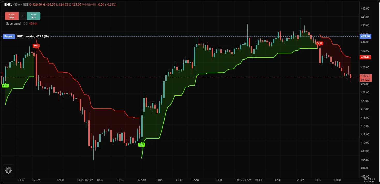
The example plots the line twice, once per direction, so each flip leaves a gap instead of a vertical jump across the candles. The flip tests compare with dir[1], which is absent on the line's first bar; == against an absent value is false, so no flip is marked there.
Remarks. The raw bands are hl2 + factor * atr(atrLen) and hl2 - factor * atr(atrLen). From bar to bar the lower band may only rise, unless the previous close fell below it, and the upper band may only fall, unless the previous close rose above it.
The line starts on the upper band, so on a rising chart the first values can read short (1) until the first close above that band flips it. While it follows the upper band it stays there as long as the close is at or below that band; while it follows the lower band it stays as long as the close is at or above it. An exact touch therefore does not flip it.
The first value arrives one bar after atr() has one, on bar atrLen, because the bands need a previous band and a previous close to trail against.
See also. psar(), atr(), barColor(), signal()
psar()
The parabolic stop and reverse: a stop that starts at the last swing extreme and moves toward price a little faster each time the trend makes a new extreme. When price reaches the stop, the trend is taken to have reversed and the stop jumps to the other side. It returns [sar, direction], with direction -1 while long and 1 while short, the same convention as supertrend().
psar(start?: number = 0.02, step?: number = 0.02, max?: number = 0.2) -> array<number>| Parameter | Type | Default | Notes |
|---|---|---|---|
start | number | 0.02 | |
step | number | 0.02 | |
max | number | 0.2 |
- Returns
array<number>- First value
- element 0 at bar 1, element 1 at bar 1
version 1
study("Parabolic SAR", overlay = true)

p   = psar(0.02, 0.02, 0.2)
sar = p[0]
dir = p[1]

plot(dir == -1 ? sar : none, "SAR, long", lime, style = "lineWithMarkers")
plot(dir == 1 ? sar : none, "SAR, short", red, style = "lineWithMarkers")

if dir == -1 and dir[1] == 1
    signal("SAR LONG", color = lime, at = "below")
if dir == 1 and dir[1] == -1
    signal("SAR SHORT", color = red, at = "above")
Remarks. It is seeded on bar 1: the direction is up if bar 1 closed above bar 0, and the stop starts at bar 0's low when up or its high when down. The acceleration starts at start.
On each later bar, in this order:
- The stop moves toward the extreme:
stop + acceleration * (extreme - stop). - If a long stop is now above the bar's low (or a short stop below its high), the direction flips, the stop jumps to the extreme the old trend reached, and the acceleration returns to
start. - Otherwise, a new extreme (a higher high while long, a lower low while short) raises the acceleration by
step, up tomax.
The stop is reported as computed: it is not pulled back outside the previous two bars' range, as some published versions do. A study that wants that clamp writes it itself.
See also. supertrend(), atr(), Exits and brackets
adx()
The average directional index and its two directional indicators. +DI measures how much of recent movement was upward and -DI how much was downward, each as a percentage of the true range. ADX measures how far apart they are, smoothed: the strength of the trend, whichever way it runs. It returns [adx, plusDI, minusDI].
adx(diLen?: number = 14, adxLen?: number = 14) -> array<number>| Parameter | Type | Default | Notes |
|---|---|---|---|
diLen | number | 14 | |
adxLen | number | 14 |
- Returns
array<number>- First value
- element 1 and 2 at bar
diLen, element 0 at bardiLen + adxLen - 1
version 1
study("ADX and DI", precision = 2)

diLen  = input(14, "DI length", min = 1, max = 100)
adxLen = input(14, "ADX smoothing", min = 1, max = 100)

a = adx(diLen, adxLen)

plot(a[0], "ADX", orange, width = 2)
plot(a[1], "+DI", lime)
plot(a[2], "-DI", red)
level(25, "Trending", fade(gray, 40), "dotted")
level(20, "Weak", fade(gray, 60), "dotted")
An ADX above about 25 and rising is commonly read as a trending market, and one below 20 as a weak or sideways one. ADX says how strong the trend is, not which way it runs: for the direction, compare the two DI lines. +DI above -DI says buyers own the move.
Remarks. Upward movement is high - high[1] and downward movement is low[1] - low; on each bar only the larger one counts, and only if it is positive. Both movements and the true range are smoothed with rma() over diLen, and each DI is smoothed movement / smoothed range * 100. ADX is the rma() over adxLen of abs(+DI - -DI) / (+DI + -DI) * 100. The two DI lines start on bar diLen (bar 14 by default) because movement needs the previous bar, and ADX starts on bar diLen + adxLen - 1 (bar 27). The DI values are absent where the smoothed range is zero, and the ratio inside ADX counts as 0 on a bar where both DI values are zero.
See also. aroon(), chop(), rma(), trueRange()
aroon()
Aroon measures how recently the window's highest high and lowest low were set, as a percentage. Aroon up is 100 when this bar set the high and falls toward 0 as the high ages; Aroon down does the same for the low. It returns [up, down]. A strong uptrend keeps Aroon up near 100 and Aroon down low.
aroon(len?: number = 14) -> array<number>| Parameter | Type | Default | Notes |
|---|---|---|---|
len | number | 14 |
- Returns
array<number>- First value
- both elements at bar
len
version 1
study("Aroon", precision = 2, range = [0, 100])

len = input(25, "Length", min = 1, max = 200)

ar = aroon(len)

plot(ar[0], "Aroon up", lime, width = 2)
plot(ar[1], "Aroon down", red, width = 2)
level(70, "Strong", fade(gray, 40), "dotted")
level(30, "Weak", fade(gray, 40), "dotted")
Remarks. Each line is 100 * (len - bars since the extreme) / len, measured over a window of len + 1 bars so that an extreme set exactly len bars ago still counts and a reading of 0 is possible. That extra bar is why the first value is on bar len. When two bars share the extreme, the more recent one counts. The Aroon oscillator is simply ar[0] - ar[1].
See also. adx(), highestBars(), lowestBars()
ichimoku()
The Ichimoku cloud: five lines that together describe trend, support and momentum. The conversion and base lines are the midpoints of the highest high and lowest low over 9 and 26 bars. Span A is the average of those two, span B is the 52 bar midpoint, and the space between the spans forms the cloud. The lagging line is the close. It returns [conversion, base, spanA, spanB, lagging].
ichimoku(
    convLen?: number = 9,
    baseLen?: number = 26,
    spanLen?: number = 52
) -> array<number>| Parameter | Type | Default | Notes |
|---|---|---|---|
convLen | number | 9 | |
baseLen | number | 26 | |
spanLen | number | 52 |
- Returns
array<number>- First value
- element by element at bar
convLen - 1,baseLen - 1,baseLen - 1,spanLen - 1,baseLen - 1
version 1
study("Ichimoku cloud", overlay = true)

ich = ichimoku(9, 26, 52)

plot(ich[0], "Conversion", aqua)
plot(ich[1], "Base", maroon)
spanA = plot(ich[2], "Span A", lime, offset = 26)
spanB = plot(ich[3], "Span B", red, offset = 26)
fill(spanA, spanB, colorUp = fade(lime, 85), colorDown = fade(red, 85))
plot(ich[4], "Lagging", gray, offset = -26)
The spans come back on the bar they are computed on, not shifted. The plot's offset draws them 26 bars forward and the lagging line 26 bars back, which is how the cloud is traditionally shown. If you change baseLen, change the offsets to match. To compare today's close with the part of the cloud drawn above today's bar, read the spans 26 bars back:
version 1
study("Close above the cloud", overlay = true)

ich   = ichimoku()
spanA = ich[2]
spanB = ich[3]

cloudTop = max(spanA[26], spanB[26])

background(close > cloudTop ? fade(lime, 92) : none)
Remarks. Each value has its own first bar: conversion on bar convLen - 1, base, span A and lagging on bar baseLen - 1, and span B on bar spanLen - 1 (bars 8, 25 and 51 with the defaults). Span A is the average of the conversion and base values, not a midpoint over a window of its own. Returning the spans unshifted means you can compare them with anything else in the script directly.
See also. donchian(), plot(), Fills
chop()
The choppiness index, a 0 to 100 reading of whether the window trended or went sideways. It compares the distance price travelled bar by bar with the range it covered overall: a market that went straight up travels about its range and reads low, while one that went back and forth travels many times its range and reads high. Use it as a filter to switch between trend-following and range-trading rules.
chop(len?: number = 14) -> series number| Parameter | Type | Default | Notes |
|---|---|---|---|
len | number | 14 |
- Returns
series number- First value
- bar
len
version 1
study("Choppiness", precision = 2, range = [0, 100])

len = input(14, "Length", min = 2, max = 200)
c = chop(len)

plot(c, "Choppiness", silver, width = 2)
level(61.8, "Choppy", fade(red, 40))
level(38.2, "Trending", fade(lime, 40))
Remarks. The reading is 100 * log10(sum of true range / (highest high - lowest low)) / log10(len). Readings above 61.8 are commonly taken as choppy and below 38.2 as trending. Each true range here needs the previous close, so the first value is on bar len rather than len - 1. The result is absent when the range or the travelled distance is not above zero, and for a length of 1.
See also. adx(), trueRange(), atr()
Oscillators and momentum
Oscillators turn price into a bounded or centred reading that is easy to compare with fixed levels: overbought and oversold, above or below zero. They are usually drawn in their own pane below the price chart, so the examples leave overlay at its default of false.
An oscillator that measures change needs two bars for its first change, so it carries one extra bar of warmup. rsi() with a length of 14 needs 14 changes, and its first value is on bar 14, not bar 13.
rsi()
The relative strength index: a 0 to 100 reading of how one-sided the recent changes were. It averages the up moves and the down moves separately and compares them. Readings above 70 are traditionally overbought and below 30 oversold, and many traders watch the 50 line as the boundary between bullish and bearish momentum.
rsi(src: series number, len?: number = 14) -> series number| Parameter | Type | Default | Notes |
|---|---|---|---|
src | series number | required | |
len | number | 14 |
- Returns
series number- First value
- bar
len
version 1
study("RSI", precision = 2, range = [0, 100])

len = input(14, "Length", min = 1, max = 200)
r = rsi(close, len)

plot(r, "RSI", purple, width = 2)
level(70, "Overbought", fade(red, 40))
level(50, "Middle", fade(gray, 60))
level(30, "Oversold", fade(lime, 40))

if crossUp(r, 30)
    alert("RSI crossed back above 30", id = "rsi-oversold-exit")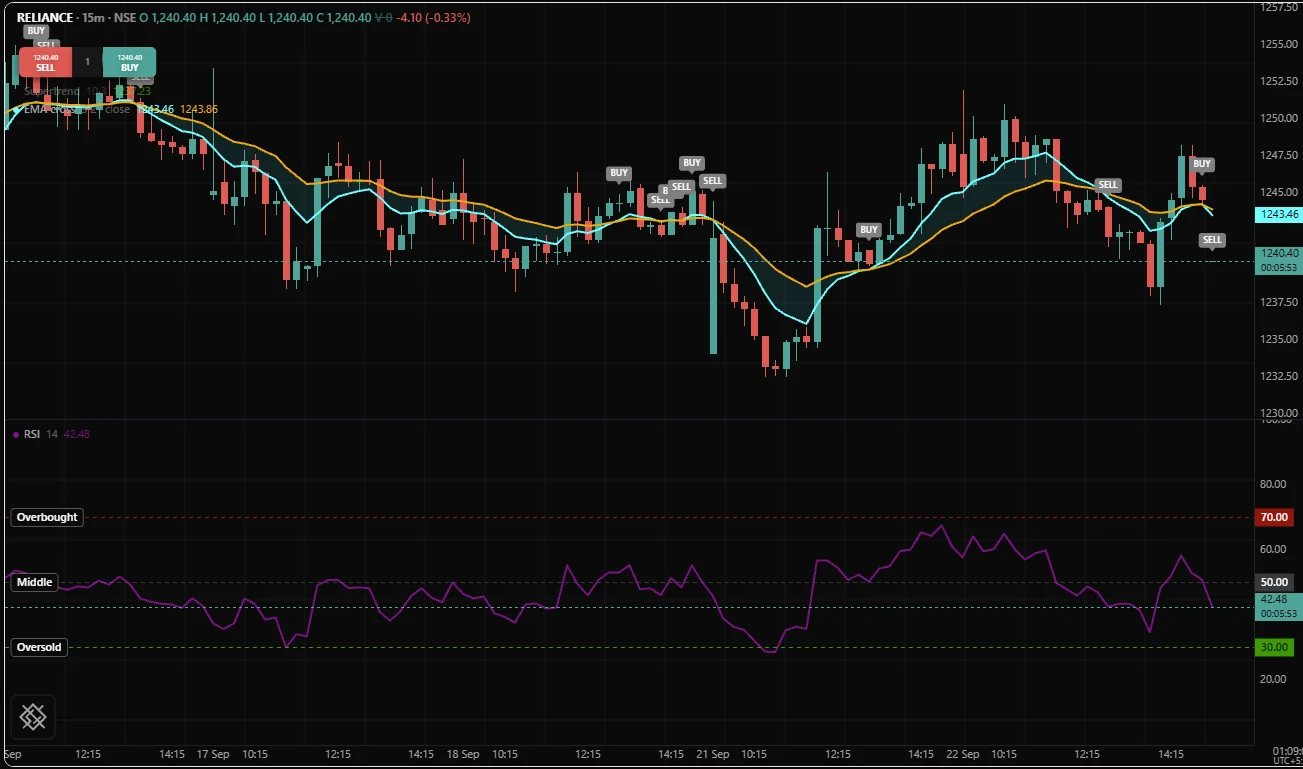
Remarks. Each change src - src[1] is split into a gain and a loss, each is smoothed with rma() over len, and the result is 100 - 100 / (1 + averageGain / averageLoss). When the average loss is zero, including a window where price never moved, the result is 100. The example under rma() rebuilds it step by step. RSI of RSI, or RSI of any series, works the same way: pass the series as src.
See also. stochRsi(), mfi(), cmo(), rma(), level()
stoch()
The stochastic oscillator places the close inside the window's range: 100 at the highest high, 0 at the lowest low. It returns [k, d], where %K is the position smoothed over smoothK bars and %D is %K smoothed over smoothD bars. With smoothK of 1 you get the fast stochastic; 3 gives the common slow stochastic.
stoch(len?: number = 14, smoothK?: number = 1, smoothD?: number = 3) -> array<number>| Parameter | Type | Default | Notes |
|---|---|---|---|
len | number | 14 | |
smoothK | number | 1 | |
smoothD | number | 3 |
- Returns
array<number>- First value
- element 0 at bar
len + smoothK - 2, element 1 at barlen + smoothK + smoothD - 3
version 1
study("Slow stochastic", precision = 2, range = [0, 100])

s = stoch(14, 3, 3)
k = s[0]
d = s[1]

plot(k, "%K", aqua, width = 2)
plot(d, "%D", orange)
level(80, "Overbought", fade(red, 40))
level(20, "Oversold", fade(lime, 40))

if crossUp(k, d) and k < 20
    signal("K UP", color = lime, at = "below", shape = "triangleUp")
Remarks. The raw position is 100 * (close - lowest low) / (highest high - lowest low) over len bars, using the bars' own highs and lows rather than the highest and lowest close. %K is sma() of that over smoothK and %D is sma() of %K over smoothD. With stoch(14, 3, 3), %K starts on bar 15 and %D on bar 17. The position is absent on a bar where the window's high equals its low.
See also. stochRsi(), williamsR(), donchian()
stochRsi()
The stochastic RSI applies the stochastic position test to rsi() instead of to price: where does today's RSI sit within its own recent range? It moves faster than RSI and reaches its extremes far more often, so it suits short-term timing. It returns [k, d].
stochRsi(
    src: series number,
    rsiLen?: number = 14,
    stochLen?: number = 14,
    smoothK?: number = 3,
    smoothD?: number = 3
) -> array<number>| Parameter | Type | Default | Notes |
|---|---|---|---|
src | series number | required | |
rsiLen | number | 14 | |
stochLen | number | 14 | |
smoothK | number | 3 | |
smoothD | number | 3 |
- Returns
array<number>- First value
- element 0 at bar
rsiLen + stochLen + smoothK - 2
version 1
study("Stochastic RSI", precision = 2, range = [0, 100])

s = stochRsi(close, 14, 14, 3, 3)

plot(s[0], "%K", aqua, width = 2)
plot(s[1], "%D", orange)
level(80, "High", fade(red, 40))
level(20, "Low", fade(lime, 40))
Remarks. The window's high and low are taken from the RSI values themselves, over stochLen bars. %K starts on bar rsiLen + stochLen + smoothK - 2 and %D follows smoothD - 1 bars later: bars 29 and 31 with the defaults. When RSI makes a new high for the window on bar after bar, the raw reading sits at 100 (and at 0 for a run of new lows), so %K can stay pinned at an extreme through a steady trend. The raw reading is absent when RSI has not moved across the window, since its high then equals its low.
williamsR()
Williams %R is the stochastic position on an inverted scale: 0 when the close is at the window's highest high and -100 at its lowest low. Readings above -20 are commonly called overbought and below -80 oversold.
williamsR(len?: number = 14) -> series number| Parameter | Type | Default | Notes |
|---|---|---|---|
len | number | 14 |
- Returns
series number- First value
- bar
len - 1
version 1
study("Williams %R", precision = 2, range = [-100, 0])

len = input(14, "Length", min = 1, max = 200)

plot(williamsR(len), "%R", red, width = 2)
level(-20, "Overbought", fade(red, 40))
level(-80, "Oversold", fade(lime, 40))
Remarks. It is computed as -100 * (highest high - close) / (highest high - lowest low), from the distance below the window high. It reads levels, not changes, so the first value is on bar len - 1. It is absent where the window's high equals its low.
See also. stoch(), stochRsi()
cci()
The commodity channel index measures how far the typical price, hlc3, sits from its own average, in units of its usual deviation. Readings beyond +100 or -100 mark a price that has moved unusually far from its mean, which traders read either as the start of a strong move or as stretched, depending on context.
cci(len?: number = 20) -> series number| Parameter | Type | Default | Notes |
|---|---|---|---|
len | number | 20 |
- Returns
series number- First value
- bar
len - 1
version 1
study("CCI", precision = 2)

len = input(20, "Length", min = 2, max = 200)
c = cci(len)

plot(c, "CCI", orange, width = 2)
level(100, "+100", fade(red, 40))
level(0, "Zero", fade(gray, 60))
level(-100, "-100", fade(lime, 40))
Remarks. The reading is (typical - sma(typical, len)) / (0.015 * mean deviation), where the mean deviation is the average absolute distance of the window's typical prices from their mean. It uses the mean absolute deviation, not the standard deviation: the 0.015 constant is calibrated for it, and a standard deviation would change every reading while still drawing a plausible line. The first value is on bar len - 1.
See also. hlc3, stdev(), bbPercent()
macd()
Moving average convergence divergence: the gap between a fast and a slow ema() of the source. It returns [macd, signal, histogram]: the gap itself, an ema() of the gap, and the difference between the two. The line crossing its signal and the histogram crossing zero are the classic momentum turns.
macd(
    src: series number,
    fast?: number = 12,
    slow?: number = 26,
    signal?: number = 9
) -> array<number>| Parameter | Type | Default | Notes |
|---|---|---|---|
src | series number | required | |
fast | number | 12 | |
slow | number | 26 | |
signal | number | 9 |
- Returns
array<number>- First value
- element 0 at bar
max(fast, slow) - 1, elements 1 and 2 at barmax(fast, slow) + signal - 2
version 1
study("MACD", precision = 2)

fastLen   = input(12, "Fast", min = 1, max = 200)
slowLen   = input(26, "Slow", min = 2, max = 400)
signalLen = input(9, "Signal", min = 1, max = 100)

m    = macd(close, fastLen, slowLen, signalLen)
line = m[0]
sig  = m[1]
hist = m[2]

plot(hist, "Histogram", hist >= 0 ? fade(lime, 40) : fade(red, 40), style = "histogram")
plot(line, "MACD", aqua, width = 2)
plot(sig, "Signal", orange)
level(0, "Zero", fade(gray, 60))

if crossUp(line, sig)
    signal("MACD UP", color = lime, at = "below", shape = "triangleUp")
Remarks. The line is ema(src, fast) - ema(src, slow). The signal average is fed the line from its first value, so it seeds on the first signal values the line produced, and the histogram is line - signal as reported. With the defaults the line starts on bar 25 and the signal and histogram on bar 33. The line is in price units, so a stock near 3,000 shows a much larger MACD than one near 300; use ppo() to compare them. Give the signal line a name other than signal: that is a library function, and assigning to it is error OS2002.
ppo()
The percentage price oscillator is MACD expressed as a percentage of the slow average. Because it is scaled by price, a stock near 3,000 and one near 300 can be compared on the same axis, and so can the same stock years apart. It returns [ppo, signal, histogram].
ppo(
    src: series number,
    fast?: number = 12,
    slow?: number = 26,
    signal?: number = 9
) -> array<number>| Parameter | Type | Default | Notes |
|---|---|---|---|
src | series number | required | |
fast | number | 12 | |
slow | number | 26 | |
signal | number | 9 |
- Returns
array<number>- First value
- as
macd
version 1
study("PPO", precision = 2)

p    = ppo(close, 12, 26, 9)
hist = p[2]

plot(hist, "Histogram", hist >= 0 ? fade(lime, 40) : fade(red, 40), style = "histogram")
plot(p[0], "PPO", aqua, width = 2)
plot(p[1], "Signal", orange)
level(0, "Zero", fade(gray, 60))
Remarks. The line is 100 * (ema(src, fast) - ema(src, slow)) / ema(src, slow); the signal and histogram are formed exactly as in macd(), with the same first values.
mom()
Momentum: the change in the source over a fixed distance, src - src[len]. Positive means price is higher than it was len bars ago, and the size says by how much, in price units.
mom(src: series number, len?: number = 10) -> series number| Parameter | Type | Default | Notes |
|---|---|---|---|
src | series number | required | |
len | number | 10 |
- Returns
series number- First value
- bar
len
version 1
study("Momentum", precision = 2)

len = input(10, "Length", min = 1, max = 200)
m = mom(close, len)

plot(m, "Momentum", m >= 0 ? lime : red, style = "histogram")
level(0, "Zero", fade(gray, 60))
Remarks. The first value is on bar len, the first bar that has a value len bars behind it. It is not smoothed; tsi() is a smoothed relative of it and roc() expresses the same change as a percentage.
roc()
Rate of change: the change over len bars as a percentage of the older value. On a daily chart, roc(close, 250) is roughly the one-year return in percent, since NSE and BSE trade about 250 sessions a year.
roc(src: series number, len?: number = 9) -> series number| Parameter | Type | Default | Notes |
|---|---|---|---|
src | series number | required | |
len | number | 9 |
- Returns
series number- First value
- bar
len
version 1
study("Rate of change", precision = 2)

len = input(9, "Length", min = 1, max = 500)

plot(roc(close, len), "ROC", lime, width = 2)
level(0, "Zero", fade(gray, 60))
Remarks. The reading is 100 * (src - src[len]) / src[len], first available on bar len. It is absent where the older value is zero.
cmo()
The Chande momentum oscillator: the sum of the up moves minus the sum of the down moves over the window, divided by their total, on a scale from -100 to 100. It is not smoothed, so a turn shows on the bar it happens. Readings beyond +50 or -50 are commonly read as strong momentum.
cmo(src: series number, len?: number = 9) -> series number| Parameter | Type | Default | Notes |
|---|---|---|---|
src | series number | required | |
len | number | 9 |
- Returns
series number- First value
- bar
len
version 1
study("Chande momentum", precision = 2, range = [-100, 100])

len = input(9, "Length", min = 1, max = 200)

plot(cmo(close, len), "CMO", aqua, width = 2)
level(50, "+50", fade(red, 40))
level(0, "Zero", fade(gray, 60))
level(-50, "-50", fade(lime, 40))
Remarks. The reading is 100 * (rise - fall) / (rise + fall), where rise and fall are the window sums of the up and down changes. It is 100 when every change in the window was up and -100 when every change was down. It is absent when price did not change at all across the window. The first value is on bar len.
tsi()
The true strength index smooths the bar-to-bar change twice, then divides by the size of the change smoothed the same way. The result, between -100 and 100, is a clean reading of the direction of momentum without the noise of mom().
tsi(src: series number, longLen?: number = 25, shortLen?: number = 13) -> series number| Parameter | Type | Default | Notes |
|---|---|---|---|
src | series number | required | |
longLen | number | 25 | |
shortLen | number | 13 |
- Returns
series number- First value
- bar
longLen + shortLen - 1
version 1
study("True strength index", precision = 2)

t   = tsi(close, 25, 13)
sig = ema(t, 7)

plot(t, "TSI", teal, width = 2)
plot(sig, "Signal", orange)
level(0, "Zero", fade(gray, 60))
Remarks. The reading is 100 * ema(ema(change, longLen), shortLen) / ema(ema(abs(change), longLen), shortLen), with the long length applied first. The first value is on bar longLen + shortLen - 1, bar 37 with the defaults. A signal line is not part of the call; the example makes one with ema().
trix()
TRIX is the one-bar percentage change of a triple exponential average. The triple smoothing filters out short swings, so TRIX turns only on sustained changes of direction. The values are small, so give the study a few extra decimals.
trix(src: series number, len?: number = 18) -> series number| Parameter | Type | Default | Notes |
|---|---|---|---|
src | series number | required | |
len | number | 18 |
- Returns
series number- First value
- bar
3 * len - 2
version 1
study("TRIX", precision = 4)

len = input(18, "Length", min = 1, max = 100)
t = trix(close, len)

plot(t, "TRIX", fuchsia, width = 2)
plot(ema(t, 9), "Signal", orange)
level(0, "Zero", fade(gray, 60))
Remarks. It is 100 * (e3 - e3[1]) / e3[1], where e3 is ema(ema(ema(src, len), len), len). That is the percentage change of the average, not the change of its logarithm. The first value is on bar 3 * len - 2, bar 52 for a length of 18.
dpo()
The detrended price oscillator removes the trend from price so that shorter cycles stand out. It subtracts a moving average taken from about half a window ago, and the peaks and troughs that remain show the rhythm of the swings. Measure the bars between its peaks to estimate a cycle length.
dpo(src: series number, len?: number = 21) -> series number| Parameter | Type | Default | Notes |
|---|---|---|---|
src | series number | required | |
len | number | 21 |
- Returns
series number- First value
- bar
len + floor(len / 2)
version 1
study("Detrended price", precision = 2)

len = input(21, "Length", min = 2, max = 200)

plot(dpo(close, len), "DPO", silver, width = 2)
level(0, "Zero", fade(gray, 60))
Remarks. The reading is src - sma(src, len)[floor(len / 2) + 1]: this bar's value less the simple average as it stood floor(len / 2) + 1 bars ago. It is reported on the current bar, not drawn back in time. The first value is on bar len + floor(len / 2), bar 31 for a length of 21.
ultimateOsc()
The ultimate oscillator blends buying pressure over three windows, 7, 14 and 28 bars by default, so that no single length dominates. It reads from 0 to 100, with 70 and 30 as the usual overbought and oversold levels.
ultimateOsc(len1?: number = 7, len2?: number = 14, len3?: number = 28) -> series number| Parameter | Type | Default | Notes |
|---|---|---|---|
len1 | number | 7 | |
len2 | number | 14 | |
len3 | number | 28 |
- Returns
series number- First value
- bar
max(len1, len2, len3)
version 1
study("Ultimate oscillator", precision = 2, range = [0, 100])

u = ultimateOsc(7, 14, 28)

plot(u, "UO", orange, width = 2)
level(70, "Overbought", fade(red, 40))
level(30, "Oversold", fade(lime, 40))
Remarks. Buying pressure is close - min(low, previous close) and the bar's range is max(high, previous close) - min(low, previous close). At each length the window sum of pressure is divided by the window sum of range, and the three ratios are blended as 100 * (4 * short + 2 * middle + long) / 7, the shortest window weighted most. Both terms need the previous close, so the first value is on bar max(len1, len2, len3), bar 28 by default.
awesomeOsc()
The awesome oscillator is the difference between a 5 bar and a 34 bar simple average of the bar midpoint, hl2. It is drawn as a histogram, coloured by whether each bar is higher than the one before.
awesomeOsc(fast?: number = 5, slow?: number = 34) -> series number| Parameter | Type | Default | Notes |
|---|---|---|---|
fast | number | 5 | |
slow | number | 34 |
- Returns
series number- First value
- bar
max(fast, slow) - 1
version 1
study("Awesome oscillator", precision = 2)

ao = awesomeOsc(5, 34)

plot(ao, "AO", ao > ao[1] ? lime : red, style = "histogram")
level(0, "Zero", fade(gray, 60))
Remarks. The reading is sma(hl2, fast) - sma(hl2, slow), first available on bar max(fast, slow) - 1, bar 33 by default.
fisher()
The Fisher transform will reshape the close's position in its recent range so that extremes stand out sharply, returning [fisher, trigger].
Named in the language and not available in version 0.5.0. Calling it is error OS2020.
fisher(len?: number = 9) -> array<number>| Parameter | Type | Default | Notes |
|---|---|---|---|
len | number | 9 |
- Returns
array<number>- First value
- bar
len
rvi()
The relative vigor index will measure where the close sits inside each bar's range, smoothed, returning [rvi, signal].
Named in the language and not available in version 0.5.0. Calling it is error OS2020.
rvi(src: series number, len?: number = 10) -> array<number>| Parameter | Type | Default | Notes |
|---|---|---|---|
src | series number | required | |
len | number | 10 |
- Returns
array<number>- First value
- bar
len + 3
coppock()
The Coppock curve will be a weighted average of two rates of change, a slow momentum turn traditionally read on monthly charts of an index.
Named in the language and not available in version 0.5.0. Calling it is error OS2020.
coppock(
    src: series number,
    roc1?: number = 14,
    roc2?: number = 11,
    wmaLen?: number = 10
) -> series number| Parameter | Type | Default | Notes |
|---|---|---|---|
src | series number | required | |
roc1 | number | 14 | |
roc2 | number | 11 | |
wmaLen | number | 10 |
- Returns
series number- First value
- bar
max(roc1, roc2) + wmaLen - 1
Volatility and bands
Volatility measures how far an instrument moves. You use it to size stops and positions, to set bands around price, and to spot quiet periods that often come before large moves.
trueRange()
True range is the bar's full range including any gap from the previous close: the largest of high - low, abs(high - previous close) and abs(low - previous close). It is the building block of atr(), and on NSE, where most gaps happen at the 09:15 open, it captures the overnight move that high - low misses.
trueRange() -> series number- Returns
series number- First value
- bar 0
version 1
study("True range and gaps", precision = 2)

tr     = trueRange()
gapped = tr > high - low

plot(tr, "True range", gapped ? orange : silver, style = "column")
When the true range is larger than the bar's own range, the previous close lay outside this bar: price gapped. The example colours those bars orange.
Remarks. On the chart's first bar there is no previous close, so the result there is high - low. This is the one deliberate exception in the library to absence spreading from a missing value: the bar's own range is a true statement about that bar, and it lets atr() start on bar len - 1.
atr()
The average true range is the rma() of trueRange(): the typical distance this instrument moves in one bar, in its own price units. It is the working measure for stop distances, target distances and position sizes.
atr(len?: number = 14) -> series number| Parameter | Type | Default | Notes |
|---|---|---|---|
len | number | 14 |
- Returns
series number- First value
- bar
len - 1
version 1
study("ATR stop levels", overlay = true)

len  = input(14, "ATR length", min = 1, max = 100)
mult = input(2.0, "Multiple", min = 0.5, max = 10, step = 0.5)

a = atr(len)

plot(close - mult * a, "Long stop", fade(red, 30), style = "step")
plot(close + mult * a, "Short stop", fade(lime, 30), style = "step")
Remarks. Because true range has a value on bar 0, the first value is on bar len - 1. The value is in price units, rupees for an NSE stock and index points for an index future, so a 2 ATR stop on a NIFTY future and on a stock are very different amounts. To size a position so every trade risks the same amount, divide the amount by the stop distance; see Position and sizing.
See also. natr(), trueRange(), supertrend(), keltner()
natr()
The normalised average true range is atr() as a percentage of the close. It lets you compare volatility between instruments at different prices, or the same instrument across years.
natr(len?: number = 14) -> series number| Parameter | Type | Default | Notes |
|---|---|---|---|
len | number | 14 |
- Returns
series number- First value
- bar
len - 1
version 1
study("ATR percent", precision = 2)

hot = input(3.0, "High volatility above, percent", min = 0.1, max = 20)
n   = natr(14)

plot(n, "ATR %", n > hot ? orange : aqua, width = 2)
level(hot, "Threshold", fade(gray, 50))
Remarks. The reading is 100 * atr(len) / close, with the same first value as atr().
stdev()
The standard deviation of the last len values: how widely they are spread around their mean, in the source's own units. By default it divides by len (the population form, which is what the band indicators use); pass sample = true to divide by len - 1. A second form takes an array and returns the standard deviation of its elements.
stdev(src: series number, len: number, sample?: bool = false) -> series number
stdev(arr: array<number>) -> number| Parameter | Type | Default | Notes |
|---|---|---|---|
src | series number | required | |
len | number | required | |
sample | bool | false | |
arr | array<number> | required |
- Returns
series number | number- First value
- bar
len - 1
version 1
study("Z-score", precision = 2)

len = input(20, "Length", min = 2, max = 500)

mean = sma(close, len)
dev  = stdev(close, len)
z    = dev > 0 ? (close - mean) / dev : none

plot(z, "Z-score", aqua, width = 2)
level(2, "+2", fade(red, 40))
level(0, "Mean", fade(gray, 60))
level(-2, "-2", fade(lime, 40))
The z-score says how many standard deviations the close sits from its average. The array form works on any list you build:
version 1
study("Spread of the last five closes", precision = 2)

closes = [close, close[1], close[2], close[3], close[4]]

plot(stdev(closes), "Deviation of five closes", silver)
Remarks. The series form computes the mean first and then the squared distances from it, in two passes, which stays accurate on prices where the values are large and the spread is small. The first value is on bar len - 1. The array form always uses the population divisor and returns none for an empty array or one holding an absent element.
See also. variance(), bollinger(), hv(), Collections
variance()
The variance of the last len values: the square of stdev(). It is in squared units (rupees squared for a price), which makes it hard to read on a chart but useful in calculations that add or compare spreads. sample = true switches to the len - 1 divisor.
variance(src: series number, len: number, sample?: bool = false) -> series number| Parameter | Type | Default | Notes |
|---|---|---|---|
src | series number | required | |
len | number | required | |
sample | bool | false |
- Returns
series number- First value
- bar
len - 1
version 1
study("Variance, population and sample", precision = 4)

len = input(20, "Length", min = 2, max = 500)

plot(variance(close, len), "Population", silver)
plot(variance(close, len, sample = true), "Sample", orange)
Remarks. It is computed in two passes, the mean first and then the squared deviations from it, so it never comes out negative. The first value is on bar len - 1. With sample = true and a length of 1 there is nothing to divide by, and the result is absent.
See also. stdev(), covariance()
hv()
Historical volatility: the standard deviation of the bar-to-bar log returns, annualised. It is the realised counterpart of an option's implied volatility, so comparing the two on NIFTY or BANKNIFTY tells you whether options are pricing more or less movement than the index has actually shown. On Indian index options the implied side of that comparison comes from Black-76 pricing off the synthetic future; hv() gives you the realised side.
hv(
    src: series number,
    len?: number = 20,
    periodsPerYear?: number = 252
) -> series number| Parameter | Type | Default | Notes |
|---|---|---|---|
src | series number | required | |
len | number | 20 | |
periodsPerYear | number | 252 |
- Returns
series number- First value
- bar
len
version 1
study("Historical volatility", precision = 2)

len     = input(20, "Length", min = 2, max = 500)
periods = input(252, "Bars per year", min = 1)

plot(hv(close, len, periods) * 100, "HV %", purple, width = 2)
Remarks. The reading is stdev(log(src / src[1]), len) * sqrt(periodsPerYear), with the population deviation. It is a proportion, not a percentage: 0.18 means 18 percent a year, so the example multiplies by 100 at the plot. periodsPerYear is the number of the chart's bars in a year: 252 for daily bars, and for intraday NSE bars the bars in the 09:15 to 15:30 session times the sessions, for example 75 * 252 (18900) on a 5-minute chart. A log return needs the previous bar, so the first value is on bar len.
bollinger()
Bollinger Bands: a simple moving average with bands a multiple of the standard deviation above and below it. The bands widen when price becomes volatile and narrow when it calms. It returns [basis, upper, lower].
bollinger(src: series number, len?: number = 20, mult?: number = 2) -> array<number>| Parameter | Type | Default | Notes |
|---|---|---|---|
src | series number | required | |
len | number | 20 | |
mult | number | 2 |
- Returns
array<number>- First value
- all elements at bar
len - 1
version 1
study("Bollinger Bands", overlay = true)

len  = input(20, "Length", min = 2, max = 500)
mult = input(2.0, "Deviations", min = 0.5, max = 5, step = 0.5)

bb = bollinger(close, len, mult)

plot(bb[0], "Basis", orange)
upper = plot(bb[1], "Upper", aqua)
lower = plot(bb[2], "Lower", aqua)
fill(upper, lower, fade(aqua, 92))
Bollinger Bands with the same settings on a BHEL 15 minute chart, from the Bollinger Bands study in Example scripts, which draws the bands in blue and labels each close that crosses outside a band:
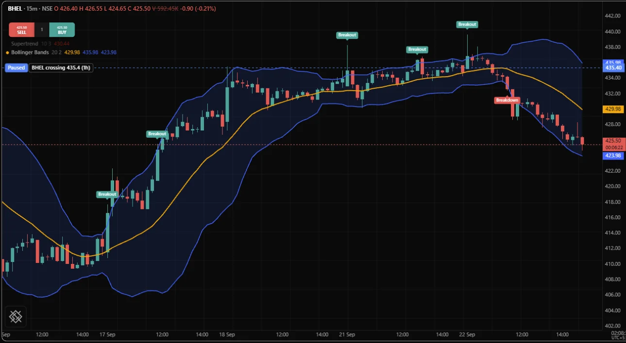
Remarks. The basis is sma(src, len), and the bands are basis + mult * stdev(src, len) and basis - mult * stdev(src, len), with the population deviation. All three values start on bar len - 1.
See also. bbWidth(), bbPercent(), keltner(), stdev()
bbWidth()
Bollinger band width: the distance between the bands divided by the basis. It turns the bands' shape into a single number, so a squeeze, the narrow and quiet stretch that often comes before a large move, shows up as a low.
bbWidth(src: series number, len?: number = 20, mult?: number = 2) -> series number| Parameter | Type | Default | Notes |
|---|---|---|---|
src | series number | required | |
len | number | 20 | |
mult | number | 2 |
- Returns
series number- First value
- bar
len - 1
version 1
study("Band width squeeze", precision = 4)

len      = input(20, "Length", min = 2, max = 500)
lookback = input(120, "Squeeze lookback", min = 10, max = 1000)

w       = bbWidth(close, len, 2)
squeeze = w <= lowest(w, lookback)

plot(w, "Band width", squeeze ? orange : aqua, width = 2)
Remarks. The reading is (upper - lower) / basis, computed from the bands exactly as bollinger() reports them, so a study that plots both agrees to the last digit. A value of 0.05 means the bands are 5 percent of the basis apart. The first value is on bar len - 1.
See also. bollinger(), bbPercent(), keltner()
bbPercent()
Percent B says where the source sits between the Bollinger Bands: 0 at the lower band, 0.5 at the basis and 1 at the upper band. It goes above 1 or below 0 when price closes outside the bands.
bbPercent(src: series number, len?: number = 20, mult?: number = 2) -> series number| Parameter | Type | Default | Notes |
|---|---|---|---|
src | series number | required | |
len | number | 20 | |
mult | number | 2 |
- Returns
series number- First value
- bar
len - 1
version 1
study("Percent B", precision = 2)

pb = bbPercent(close, 20, 2)

plot(pb, "%B", aqua, width = 2)
level(1, "Upper band", fade(red, 40))
level(0.5, "Basis", fade(gray, 60))
level(0, "Lower band", fade(lime, 40))
Remarks. The reading is (src - lower) / (upper - lower), from the bands as reported. It is absent on a bar where the bands meet: when every value in the window is equal, or when mult is 0. The first value is on bar len - 1.
See also. bollinger(), bbWidth(), stoch()
keltner()
Keltner channels: a moving average of the close with bands a multiple of the average true range above and below it. Where Bollinger Bands widen with the spread of closes, Keltner channels widen with how far the bars actually travel, which makes them steadier. It returns [basis, upper, lower].
keltner(
    len?: number = 20,
    mult?: number = 2,
    atrLen?: number = 10,
    maType?: string = "ema"
) -> array<number>| Parameter | Type | Default | Notes |
|---|---|---|---|
len | number | 20 | |
mult | number | 2 | |
atrLen | number | 10 | |
maType | string | "ema" |
- Returns
array<number>- First value
- all elements at bar
max(len, atrLen) - 1
version 1
study("Keltner channel and squeeze", overlay = true)

len  = input(20, "Length", min = 2, max = 500)
mult = input(1.5, "ATR multiple", min = 0.5, max = 5, step = 0.25)

kc = keltner(len, mult, 10, "ema")
bb = bollinger(close, len, 2)

plot(kc[0], "Basis", orange)
upper = plot(kc[1], "Upper", teal)
lower = plot(kc[2], "Lower", teal)
fill(upper, lower, fade(teal, 92))

squeezed = bb[1] < kc[1] and bb[2] > kc[2]
background(squeezed ? fade(yellow, 90) : none)
The background marks a squeeze: the Bollinger Bands sitting inside the Keltner channel. During warmup either side of the comparison is absent, the condition takes the false branch, and nothing is painted.
Remarks. The basis is the average of the close over len, of the type maType names: "sma", "ema", "wma", "rma", "hma" or "vwma", as in ma(). The width is atr(atrLen), and the bands are basis + mult * atr and basis - mult * atr. All three values start on bar max(len, atrLen) - 1. The compiler does not check maType; a name that is not one of the six leaves all three values absent on every bar.
See also. bollinger(), atr(), ma(), donchian()
donchian()
Donchian channels: the highest high and lowest low of the last len bars, with the midpoint between them. A close beyond the previous bar's channel is a breakout, the basis of many trend-following systems. It returns [upper, basis, lower], upper first.
donchian(len?: number = 20) -> array<number>| Parameter | Type | Default | Notes |
|---|---|---|---|
len | number | 20 |
- Returns
array<number>- First value
- all elements at bar
len - 1
version 1
study("Donchian breakout", overlay = true)

len = input(20, "Length", min = 2, max = 500)

dc    = donchian(len)
upper = dc[0]
lower = dc[2]

plot(upper, "Upper", lime, style = "step")
plot(dc[1], "Middle", fade(gray, 40), style = "step")
plot(lower, "Lower", red, style = "step")

if close > upper[1]
    signal("BREAKOUT", color = lime, at = "below", shape = "triangleUp")
if close < lower[1]
    signal("BREAKDOWN", color = red, at = "above", shape = "triangleDown")
Remarks. The window includes the current bar, so the close can never be above this bar's upper line. Test a breakout against the previous bar's channel, upper[1], as the example does. The middle value is (upper + lower) / 2. All three start on bar len - 1.
See also. highest(), lowest(), keltner(), ichimoku()
massIndex()
The mass index will measure how much the high to low range is expanding, as a warning that a trend may be about to reverse.
Named in the language and not available in version 0.5.0. Calling it is error OS2020.
massIndex(len?: number = 25) -> series number| Parameter | Type | Default | Notes |
|---|---|---|---|
len | number | 25 |
- Returns
series number- First value
- bar
len + 17
Volume
Volume indicators ask whether traders are backing a price move with size. They need the traded volume of each bar, which the host (the application running the script, such as the /trading chart) supplies with the price. An index itself, such as NIFTY 50 or BANKNIFTY, trades no volume, so these functions have nothing to measure on an index chart: chart the index future on NFO when you need volume for an index. On a bar whose volume is absent, every function in this section is absent too.
vwap()
The volume weighted average price since the session opened: the average price paid for every unit traded today. Intraday traders use it as the day's fair value: price above VWAP favours buyers, below favours sellers. It restarts on the first bar of each trading session, found from the session hours the host states for the instrument (09:15 IST for NSE and NFO), not at midnight.
vwap(src?: series number = hlc3) -> series number| Parameter | Type | Default | Notes |
|---|---|---|---|
src | series number | hlc3 |
- Returns
series number- First value
- the session's first bar
version 1
study("Session VWAP", overlay = true)

v = vwap()

plot(v, "VWAP", orange, width = 2)
barColor(close > v ? lime : close < v ? red : none)No Indian session runs past midnight IST, so a new IST date is a new session. Anchoring vwapAnchor() to that gives the same average, and it works on the /trading chart today:
version 1
study("Day VWAP by the IST date", overlay = true)

// A new trading day: the first bar on the chart, or a bar on a different
// IST date from the bar before it.
newDay = isNone(time[1]) or not date.isSameDay(time, time[1], "Asia/Kolkata")

dayVwap = vwapAnchor(hlc3, newDay)

plot(dayVwap, "Day VWAP", orange, width = 2)
barColor(close > dayVwap ? lime : close < dayVwap ? red : none)
Remarks. It is sum(src * volume) / sum(volume) over the session so far, with src defaulting to hlc3. Both running totals restart on the session's first bar before that bar is added, so the first bar of each session is the first bar of the new average. On a daily or longer chart every bar is its own session and the result equals src; the compiler does not warn about that yet. A bar with absent data gives an absent result and leaves the totals as they were.
See also. vwapAnchor(), vwma(), session.isFirstBar, Sessions and time
vwapAnchor()
The same volume weighted average, restarted on every bar where resetWhen is true. Anchor it to the start of a week, a month, an expiry, a result announcement or any condition you can write.
vwapAnchor(src: series number, resetWhen: series bool) -> series number| Parameter | Type | Default | Notes |
|---|---|---|---|
src | series number | required | |
resetWhen | series bool | required |
- Returns
series number- First value
- the first bar
resetWhenis true
version 1
study("Weekly and monthly VWAP", overlay = true)

newWeek  = date.startOfWeek(time) != date.startOfWeek(time[1])
newMonth = date.month(time) != date.month(time[1])

plot(vwapAnchor(hlc3, newWeek), "Weekly VWAP", aqua, width = 2)
plot(vwapAnchor(hlc3, newMonth), "Monthly VWAP", fuchsia, width = 2)
The conditions compare this bar's week and month with the previous bar's, so a week whose Monday is a market holiday still resets on its first trading day.
Remarks. The result is absent until resetWhen is first true, because there is no anchor to measure from. On an anchor bar both totals are reset before the bar's own price and volume are added, so the anchor bar opens the new average. On the chart's first bar time[1] is absent and != is true, so the example's first average starts there.
See also. vwap(), date.startOfWeek(), date.month()
obv()
On balance volume: a running total that adds the bar's whole volume when the close rises and subtracts it when the close falls. The level means little on its own; what matters is its direction and whether it confirms price. A price high that on balance volume does not confirm is a warning.
obv() -> series number- Returns
series number- First value
- bar 0, seeded 0
version 1
study("On balance volume", format = "volume")

o = obv()

plot(o, "OBV", teal, width = 2)
plot(ema(o, 20), "OBV average", fade(orange, 30))
Remarks. The total starts at 0 on the chart's first bar, which has no earlier close to compare with. An unchanged close adds nothing. An absent bar gives an absent result and leaves the total where it was.
ad()
The accumulation distribution line: a running total of volume weighted by where the close sat inside the bar. A close at the high adds the whole volume, a close at the low subtracts it, and a close in the middle adds nothing. A rising line says the closes are landing near the highs.
ad() -> series number- Returns
series number- First value
- bar 0
version 1
study("Accumulation distribution", format = "volume")

plot(ad(), "A/D", lime, width = 2)
Remarks. Each bar adds ((close - low) - (high - close)) / (high - low) * volume. A bar with no range, where high equals low, adds 0 rather than ending the total. The total starts at 0 before the first bar.
adOsc()
The accumulation distribution oscillator, often called the Chaikin oscillator: a fast ema() of the ad() line minus a slow one. It dates the turns in accumulation, crossing above zero when buying pressure picks up.
adOsc(fast?: number = 3, slow?: number = 10) -> series number| Parameter | Type | Default | Notes |
|---|---|---|---|
fast | number | 3 | |
slow | number | 10 |
- Returns
series number- First value
- bar
max(fast, slow) - 1
version 1
study("A/D oscillator", format = "volume")

osc = adOsc(3, 10)

plot(osc, "A/D oscillator", osc >= 0 ? lime : red, style = "histogram")
level(0, "Zero", fade(gray, 60))
Remarks. It is ema(ad, fast) - ema(ad, slow), taken over the running total rather than the per-bar term. The first value is on bar max(fast, slow) - 1, bar 9 by default.
cmf()
Chaikin money flow: the accumulation over the window as a fraction of the volume traded in it. It runs from -1 to 1; readings above zero say closes have been landing in the upper half of their bars on the volume that mattered.
cmf(len?: number = 20) -> series number| Parameter | Type | Default | Notes |
|---|---|---|---|
len | number | 20 |
- Returns
series number- First value
- bar
len - 1
version 1
study("Chaikin money flow", precision = 3)

c = cmf(20)

plot(c, "CMF", c >= 0 ? lime : red, style = "histogram")
level(0.05, "Buying", fade(lime, 50), "dotted")
level(-0.05, "Selling", fade(red, 50), "dotted")
Remarks. It is the window sum of the ad() per-bar term divided by the window sum of volume, first available on bar len - 1. The plus and minus 0.05 lines are a common threshold, not part of the definition.
mfi()
The money flow index is rsi() computed on money flow, the typical price times volume, instead of on price. It reads from 0 to 100, with 80 and 20 as the usual overbought and oversold levels.
mfi(len?: number = 14) -> series number| Parameter | Type | Default | Notes |
|---|---|---|---|
len | number | 14 |
- Returns
series number- First value
- bar
len
version 1
study("Money flow index", precision = 2, range = [0, 100])

m = mfi(14)

plot(m, "MFI", purple, width = 2)
level(80, "Overbought", fade(red, 40))
level(20, "Oversold", fade(lime, 40))
Remarks. Each bar's flow is hlc3 times volume. The flow counts on the rising side when the typical price rose from the previous bar and on the falling side when it fell; an unchanged typical price counts on neither. The result is 100 - 100 / (1 + rising / falling) over window sums, not smoothed averages, and it is 100 when the falling sum is zero. The first value is on bar len.
pvt()
The price volume trend: a running total of volume weighted by the percentage change of the close. Unlike obv(), which adds the whole volume for any rise, a small rise adds a small share and a large rise a large one.
pvt() -> series number- Returns
series number- First value
- bar 1, seeded 0
version 1
study("Price volume trend", format = "volume")

p = pvt()

plot(p, "PVT", olive, width = 2)
plot(ema(p, 21), "PVT average", fade(orange, 30))
Remarks. Each bar adds (close - close[1]) / close[1] * volume to a total that starts at 0. The first bar has no change behind it and is absent; the second bar already carries its own term.
eom()
Ease of movement: how far the bar's midpoint moved per unit of volume, averaged over len bars. A large positive reading means price rose easily on light volume; a reading near zero means it took heavy volume to move price at all.
eom(len?: number = 14) -> series number| Parameter | Type | Default | Notes |
|---|---|---|---|
len | number | 14 |
- Returns
series number- First value
- bar
len
version 1
study("Ease of movement", precision = 2)

scale = input(100000, "Display scale", min = 1)
e     = eom(14) * scale

plot(e, "EOM", e >= 0 ? lime : red, width = 2)
level(0, "Zero", fade(gray, 60))
Remarks. Each bar's term is (hl2 - hl2[1]) * (high - low) / volume, and the result is its sma() over len, first available on bar len. No scaling constant is applied, so on a liquid NSE stock, where volume runs to lakhs of shares, the raw reading is very small. Multiply it at the plot to bring it into a readable range, as the example does with an input.
See also. forceIndex(), hl2
forceIndex()
The force index multiplies each bar's change in close by its volume and smooths the result: a big move on big volume is a strong force. Crossings of zero mark shifts between buying and selling pressure.
forceIndex(len?: number = 13) -> series number| Parameter | Type | Default | Notes |
|---|---|---|---|
len | number | 13 |
- Returns
series number- First value
- bar
len
version 1
study("Force index", format = "volume")

f = forceIndex(13)

plot(f, "Force", f >= 0 ? lime : red, style = "histogram")
level(0, "Zero", fade(gray, 60))
Remarks. It is the ema() over len of (close - close[1]) * volume. The first change is on bar 1, so the first value is on bar len. The values are large, so the example uses the study's volume format for the axis.
relativeVolume()
Relative volume: this bar's volume divided by its average volume over the last len bars. A reading of 2 means twice the normal volume. Use it to confirm breakouts and to spot unusual activity. On an intraday chart, the opening bars at 09:15 naturally trade far more than midday bars, so compare like with like or use a daily chart.
relativeVolume(len?: number = 20) -> series number| Parameter | Type | Default | Notes |
|---|---|---|---|
len | number | 20 |
- Returns
series number- First value
- bar
len - 1
version 1
study("Confirmed breakout", overlay = true)

len   = input(20, "Lookback", min = 2, max = 500)
ratio = input(1.8, "Volume multiple", min = 1, max = 10)

hi = highest(high, len)[1]
rv = relativeVolume(len)

plot(hi, "Breakout level", orange, style = "step")

if close > hi and rv > ratio
    signal("BREAK", color = lime, at = "below", shape = "triangleUp")
Remarks. It is volume / sma(volume, len), first available on bar len - 1. The average includes the current bar.
nvi()
The negative volume index will keep a running total of price changes on bars where volume fell, following the idea that informed traders act on quiet days.
Named in the language and not available in version 0.5.0. Calling it is error OS2020.
nvi() -> series number- Returns
series number- First value
- bar 1
pvi()
The positive volume index will keep a running total of price changes on bars where volume rose.
Named in the language and not available in version 0.5.0. Calling it is error OS2020.
pvi() -> series number- Returns
series number- First value
- bar 1
klinger()
The Klinger oscillator will compare volume force with the trend of each bar, returning [klinger, signal].
Named in the language and not available in version 0.5.0. Calling it is error OS2020.
klinger(fast?: number = 34, slow?: number = 55, signal?: number = 13) -> array<number>| Parameter | Type | Default | Notes |
|---|---|---|---|
fast | number | 34 | |
slow | number | 55 | |
signal | number | 13 |
- Returns
array<number>- First value
- bar
slow + signal - 2
cvd()
Cumulative volume delta will keep a running total of buying minus selling volume, once hosts supply the trade-by-trade data inside each bar.
Named in the language and not available in version 0.5.0. Calling it is error OS2020.
cvd() -> series number- Returns
series number- First value
- bar 0
volumeProfile()
The volume profile will total the volume traded at each price level since an anchor bar, for a histogram drawn sideways against the price axis.
Named in the language and not available in version 0.5.0. Calling it is error OS2020.
volumeProfile(rows?: number = 24, from?: number = none) -> array<number>| Parameter | Type | Default | Notes |
|---|---|---|---|
rows | number | 24 | |
from | number | none |
- Returns
array<number>- First value
- the anchor bar
Pattern and swing
Swing points mark the turns of the market: the highs and lows that define support, resistance and the structure of a trend. The dedicated swing function, zigzag(), is planned. Until it arrives, build swings from pivotHigh() and pivotLow(), which confirm a turn after a set number of bars on each side:
version 1
study("Swing highs and lows", overlay = true)

left  = input(5, "Bars to the left", min = 1, max = 50)
right = input(5, "Bars to the right", min = 1, max = 50)

ph = pivotHigh(high, left, right)
pl = pivotLow(low, left, right)

var lastHigh = none
var lastLow  = none

if not isNone(ph)
    lastHigh = ph
if not isNone(pl)
    lastLow = pl

plot(lastHigh, "Last swing high", fade(red, 30), style = "step")
plot(lastLow, "Last swing low", fade(lime, 30), style = "step")
A pivot is known only right bars after it forms, so the levels step in late by that many bars. That delay is the honest cost of confirming a swing, not a fault. Series functions documents the pivot functions in full.
zigzag()
Zigzag will connect swing highs and lows that are confirmed once price reverses by at least deviation percent, filtering out smaller moves.
Named in the language and not available in version 0.5.0. Calling it is error OS2020.
zigzag(src: series number, deviation: number) -> array<number>| Parameter | Type | Default | Notes |
|---|---|---|---|
src | series number | required | |
deviation | number | required |
- Returns
array<number>- First value
- first confirmed swing
Related
Series functions for highest(), crossUp(), change() and the other helpers these indicators are built from. Warmup and Absent values for why a line starts where it does. Plotting for drawing a result, Higher timeframes for running any indicator on a coarser interval, and Inputs for making lengths and multipliers adjustable.