
Levels
level() draws one horizontal line across a pane, for oscillator thresholds and reference prices such as the previous day's high, and the study options that fix a pane's range and format its price axis.
On this page
A level is one horizontal line straight across a pane at one price. It takes one call, costs no plot slot and keeps no history. This page covers when to use a level rather than a plot, how to compute a level from the data (the previous day's high on an intraday NIFTY chart, say), the one rule that explains everything surprising about levels, and the study options that fix a pane's range and control what its price axis says.
A first example
A relative strength index (RSI) in its own pane, with its two thresholds and a midline:
version 1
study("RSI with levels", precision = 2, range = [0, 100])

len = input(14, "Length", min = 2, max = 200)

// Declared before the plot, as reference lines for the reading.
level(70, "Overbought", fade(red, 40))
level(50, "Middle", fade(gray, 70), style = "dotted")
level(30, "Oversold", fade(lime, 40))

plot(rsi(close, len), "RSI", purple, width = 2)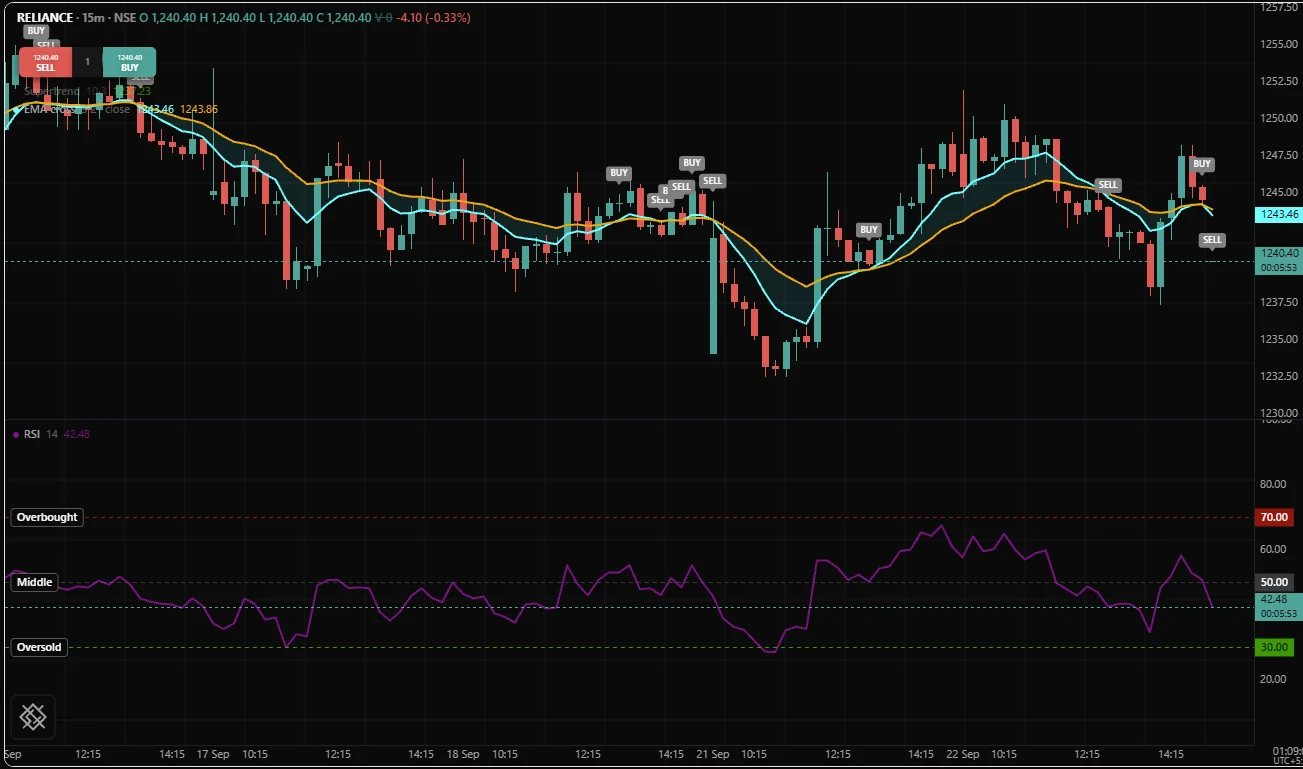
Each level is drawn as a line across the pane, with its title in a small plate at the left end of the line and its price tagged on the right-hand axis in the level's colour.
Three details are deliberate. The thresholds are faded, because they are reference and the RSI is data. The midline is dotted rather than dashed, one step further back, because it is a reference for the references. And range = [0, 100] pins the pane's scale, so 70 and 30 sit at the same height on every chart you open.
What a level is, and what it is not
A plot draws a different value on every bar. A level draws one value across the whole pane. The difference is not cosmetic:
level | plot | |
|---|---|---|
| What is drawn | One horizontal line across the pane | A column of one value per bar |
| Plot slot | None | One |
| Value in the legend | No | Yes |
| Group in the Style tab | No | Yes |
| History | None: you see one line, not where it used to be | Every bar's value is drawn at that bar |
| Price | Read every bar; the line is drawn at the last bar's value | Every bar's value is drawn at that bar |
Can a fill name it | No | Yes |
A level is the right call for a threshold a reader needs to see everywhere on the pane: 70 and 30 on an oscillator, zero under a signed histogram, the previous day's high on a price chart. It is the wrong call for anything whose past positions are part of the picture.
The call
level() takes a price and four optional arguments:
| Argument | Default | Means |
|---|---|---|
price | required | The price to draw the line at. none draws nothing |
title | "" | The label at the left end of the line. No two levels in a file may share one |
color | gray | The line colour |
style | "dashed" | "solid", "dashed" or "dotted" |
width | 1 | Thickness |
Only price is read per bar. title, color, style and width are fixed before the first bar: write them in the call, as a literal or a colour built from literals such as fade(red, 40), or pass an input() by its own name. A colour that changes from bar to bar is OS3003, and so is a colour taken from a name you computed earlier:
r = rsi(close, 14)
level(70, "Overbought", r > 70 ? red : gray)
A level whose colour the user can change takes a colour input straight into the call. To make that colour faded, put the fade in the input's default, because wrapping fade() around the input inside the call is refused:
obColor = input(fade(red, 40), "Overbought line")
level(70, "Overbought", obColor)
level declares part of the study's fixed shape, so it is top level only, like plot and fill. Inside an if it is OS3006. To make a level disappear, give it an absent price.
The default style is dashed on purpose. A reference line is not data. A solid line at 70 competes with the oscillator it is a reference for, and a reader has to work out which of the two lines is the reading. A dashed line reads as scaffolding at any distance, which is what it is.
Levels computed from the data
A level's price does not have to be a constant. It can be any expression, and it is read again on every bar. Here the previous day's range is drawn on an intraday chart of an NSE stock or index future:
version 1
study("Previous day range", overlay = true)

// The default "confirmed" mode reads only daily bars that have closed, so
// these are the previous day's numbers and they never repaint.
dayHigh = req.timeframe("1D", high)
dayLow  = req.timeframe("1D", low)
dayMid  = (dayHigh + dayLow) / 2

level(dayHigh, "Previous day high", fade(aqua, 25), width = 2)
level(dayMid,  "Previous day midpoint", fade(gray, 55), style = "dotted")
level(dayLow,  "Previous day low", fade(orange, 25), width = 2)
Three lines, no plot slots, and they move to the new day's numbers by themselves when the next session's first bar arrives. See Higher timeframes for how req.timeframe() reads a coarser interval without repainting.
A level's price counts when the chart fits the pane's scale to what is on screen, so a level far from the current price stretches the pane to keep itself in view. That is usually what you want from the previous day's high; it is a reason not to draw levels at prices nobody needs to see.
The rule that follows: the last bar wins
A level's price is evaluated on every bar, and the line drawn is the one from the last bar the script ran on.
Everything surprising about levels comes from that rule. A level has no history. There is one line, and its height is whatever the expression produced on the most recent bar. Scrolling back to last month does not show you where the level was last month; it shows the same line at today's height.
Two consequences follow, each with its fix.
If the price is absent on the last bar, no line is drawn at all. This obvious-looking line usually draws nothing, because only the day's first bar has a value and the last bar is rarely that one:
// A new trading day: the first bar on the chart, or a bar on a different IST
// date from the bar before it.
newDay = isNone(time[1]) or not date.isSameDay(time, time[1], "Asia/Kolkata")

// Absent on every bar except the day's first, so usually nothing is drawn.
level(newDay ? open : none, "Day open", aqua)
The fix is to hold the value in a var, which keeps it from one bar to the next (Persistence):
version 1
study("Day open", overlay = true)

newDay = isNone(time[1]) or not date.isSameDay(time, time[1], "Asia/Kolkata")

var dayOpen = none

// Captured on the day's first bar (09:15 on NSE) and carried on every bar
// after it, so the level has a value on whichever bar turns out to be the last.
if newDay
    dayOpen = open

level(dayOpen, "Day open", fade(aqua, 25), style = "solid", width = 2)
The first bar of the day is found here by a change of date in IST, which is right for NSE, BSE and MCX because none of their sessions runs past midnight. The language's own session.isFirstBar needs the exchange's session hours, which the /trading chart does not supply in this release, so it has no value there. Sessions and time explains both.
If you want to see where the level used to be, it is not a level. A value whose past matters is a column, and a column is a plot. Use style = "step" so the picture says "it was this, then it became that" rather than sloping between readings that never happened:
newDay = isNone(time[1]) or not date.isSameDay(time, time[1], "Asia/Kolkata")

var dayOpen = none
if newDay
    dayOpen = open

// Every past day's open, at the bars it applied to.
plot(dayOpen, "Day open", fade(aqua, 25), width = 2, style = "step")
Both forms are right; they answer different questions. The level answers "where is it now", from anywhere on the chart. The step plot answers "where was it then". A study that wants both draws both, and pays one plot slot for the second.
Choosing between a level, a step plot and a drawing
level | plot(..., style = "step") | draw.line | |
|---|---|---|---|
| Extent | The whole pane, edge to edge | The bars the value existed on | Between two anchored points, optionally extended |
| How many | Fixed when the script compiles, one per call | Fixed when the script compiles, one per call | As many as the script creates, at any time |
| Past positions | Not shown | Shown | Shown, and each one stays until deleted |
| Cost | None | One plot slot | Memory per object |
| Readable back | No | Yes, with [] | No |
| Good for | A threshold, today's reference prices, a zero line | A reference whose history matters | A trendline, a zone, a channel between two pivots |
In one sentence each: a threshold is a level, a reference with a history is a step plot, and a geometric object between two points in time is a drawing. Drawings are covered on Lines and boxes.
Fixing a pane's range
version 1
study("RSI", precision = 2, range = [0, 100])

plot(rsi(close, 14), "RSI", purple, width = 2)
range takes [min, max] and pins the study pane's scale. It is a study option, so it applies to the whole pane. Write both bounds as plain numbers, low first. An input, arithmetic such as 50 + 50, or a low that is not below the high is OS3016. Negative bounds and decimals are fine.
Why pin it at all? An unpinned pane fits its scale to the values on screen and the levels in it, so the same reading sits at a different height on every chart and at every zoom, and a quiet month is stretched to fill the pane like a dramatic one. Pinning the range fixes the heights: 70 is always the same distance from the top, and a quiet month looks quiet, which is the whole value of a bounded oscillator.
| Reading | Pin it? | Why |
|---|---|---|
| A 0 to 100 oscillator, such as RSI or stochastic | Yes, [0, 100] | It has real bounds, and the thresholds have fixed meaning |
| A -100 to 100 oscillator | Yes | The same, and zero sits in the middle of the pane |
| A 0 to 1 position within a band | Yes, or a little wider | It has real bounds, and values outside them are themselves the signal |
| A trend strength reading that lives between 10 and 40 | Yes, to the useful part | [0, 60] uses the pane; [0, 100] wastes half of it |
| A difference of two moving averages | No | It has no bounds, and its scale changes with the instrument |
| Volume, a spread, an option premium | No | The useful scale changes from week to week |
| A percentage change | Usually not | The interesting range depends on the instrument and the interval |
Pinning a range is a promise that values outside it do not need to be read: the pane cuts them off at its edge. If the reading can leave the range and you still want to see it, do not pin it.
A pinned range pairs naturally with levels: the levels give the pane fixed landmarks, and the range keeps those landmarks at the same height.
version 1
study("Position in the band", precision = 2, range = [-0.25, 1.25])

len  = input(20,  "Length", min = 2, max = 500)
mult = input(2.0, "Deviations", min = 0.1, max = 10)

// 0 at the lower band and 1 at the upper one. The range is widened a quarter
// each way, so a close outside the band is visible instead of cut off.
p = bbPercent(close, len, mult)

level(1,   "Upper band", fade(red, 40))
level(0,   "Lower band", fade(lime, 40))
level(0.5, "Basis", fade(gray, 70), style = "dotted")

plot(p, "Position", purple, width = 2)
The price axis
Four settings decide what the axis beside a study's own pane says:
| Want | Set | Where |
|---|---|---|
| How many decimals | precision, a whole number from 0 to 10 | The declaration, or a plot for the scale it maps to |
| Whether it reads as a price, a percentage or a volume | format: "price", "percent" or "volume" | The declaration, or a plot for the scale it maps to |
| Which side of the pane a column maps to | scale: "right", "left" or "none" | Each plot. The declaration accepts scale too, but the /trading chart does not apply it in this release |
| The fixed extent of the scale | range = [min, max] | The declaration |
"percent" writes the number with a percent sign after it and changes nothing else. "volume" shortens large numbers, so 1250000 reads 1.25M, and does not use precision:
version 1
study("Traded quantity", format = "volume")

plot(volume, "Volume", fade(aqua, 30), style = "column")
Set precision and format on the declaration whenever the whole pane reads the same way, which is almost always. Set on an individual plot, they format the price scale that plot maps to, not that one line, because formatting belongs to an axis and an axis is shared.
None of this reaches the price pane. There the axis is the instrument's own: an overlay study's declared precision and format are not applied to it, and in a study declared with overlay = true the compiler raises warning OS8007 for any plot that sets either one. Plots has the details.
Formatting is display only. format = "percent" multiplies nothing by a hundred and precision = 2 rounds nothing. Use round() when you want the value itself changed.
Titles and axis tags
A level's title is its label, shown at the left end of the line. Give every level a title even when the height looks obvious, because a pane with four unlabelled dashed lines is a pane whose author knew what they meant and whose reader does not.
level(70, "Overbought", fade(red, 40))       // labelled
level(30, color = fade(lime, 40))            // a line with no explanation
The right-hand axis carries tags the chart writes for you: each level's price, and the latest value of the plots on that axis, each in its own colour. When you want words beside a value, anchor a label to the newest bar and move it as new bars arrive:
version 1
study("EMA with a tag", overlay = true)

e = ema(close, 20)

var tag = none

// Only on the newest bar: one label, created once and then moved, rather
// than a new label on every bar.
if bar.isLast
    if isNone(tag)
        tag = draw.label(time, e, "EMA 20 " + text(e, 2), color = fade(orange, 25), textColor = black)
    else
        draw.setAt(tag, time, e)
        draw.setText(tag, "EMA 20 " + text(e, 2))

plot(e, "EMA 20", orange, width = 2)
That is more work than a level, and it buys something neither a level nor a plot gives: a name and a value together, beside the newest bar where a trader is reading.
Common reference lines
The ones almost every study wants:
| Line | Written |
|---|---|
| Zero, under a signed oscillator | level(0, "Zero", fade(gray, 55), style = "solid") |
| Oscillator thresholds | level(70, "Overbought", fade(red, 40)) and level(30, "Oversold", fade(lime, 40)) |
| A midline | level(50, "Middle", fade(gray, 70), style = "dotted") |
| The previous day's high and low | level(req.timeframe("1D", high), "Previous day high", fade(aqua, 25)) |
Today's open, held in a var | Capture on the day's first bar, then level(dayOpen, "Day open") |
| A price the user types | myLine = input(0.0, "My line"), then level(myLine, "My line", fade(aqua, 25)) |
| A position's average price, in a strategy | level(pos.avgPrice, "Entry", fade(silver, 30)) |
Write each input() on its own line at the top rather than nesting it inside the level call: every input is a row of the settings dialog, and a reader scanning the file wants all of them in one block.
The last row is a level whose price is absent some of the time, which is exactly right: pos.avgPrice is absent while the strategy is flat, an entry line means nothing then, and an absent price draws no line. A stop a set distance from the entry works the same way. Compute the average true range at the top level first, so its state advances on every bar:
version 1
strategy("Entry and stop", overlay = true)

mult  = input(2.0, "Stop, in ATR", min = 0.5, max = 10)

fast  = ema(close, 9)
slow  = ema(close, 21)
atr14 = atr(14)

if crossUp(fast, slow)
    buy()
if crossDown(fast, slow)
    close()

// Drawn only while a position is open on the newest bar.
level(pos.avgPrice, "Entry", fade(silver, 30))
level(pos.avgPrice - mult * atr14, "Stop", fade(red, 30))
Because the last bar wins, these two lines show the trade that is open now, and nothing between trades. To see the entry of every past trade, plot pos.avgPrice with style = "step" instead.
Common mistakes
| Mistake | What happens | Fix |
|---|---|---|
Wrapping level in an if | OS3006 | Give the price none on the bars where there is none |
| A colour that changes per bar | OS3003 | A level has one colour. Use a plot for a line whose colour changes |
fade() around a colour input inside the call | Refused when the script compiles | Put the fade in the input's default |
| A level whose price is set on one bar only | Usually nothing is drawn, because the last bar decides | Hold the value in a var |
| Expecting to scroll back and see where the level was | A level has no history | Use plot(..., style = "step") |
Trying to fill between a plot and a level | A level is not a plot and cannot be one end of a fill | Plot the constant, fully transparent if it should not show. See Fills |
An input or arithmetic in range | OS3016 | Two plain numbers, low first |
| Pinning a range on an unbounded reading | The line leaves the pane and you cannot see it | Only pin a reading with real bounds |
precision or format on a plot in an overlay study | Warning OS8007 | Leave them off over the price pane |
| Solid reference lines as heavy as the data | The reader cannot tell the reference from the reading | Dashed or dotted, faded, thin |
| Levels with no titles | Nobody else can read the pane | Title every one |
Related: Visuals overview, Plots, Fills, Lines and boxes, Declarations, Plotting reference.