
Settings and style
The study settings dialog in /trading, its Inputs and Style tabs, what a reader can restyle without any input, the declaration options that place and format a study, and what /trading keeps between visits.
On this page
Every study you put on a chart in /trading gets a settings dialog, a legend row and a place in the Indicators dialog, and your script declares none of it. The dialog is generated from two things the compiler fixes before the first bar: your input() calls, and the plots the study draws. This page walks through that dialog as it appears in /trading, explains what a reader can change without you writing a line, covers the declaration options of an OpenScript (also called OpenAlgo Script) study, and says what /trading keeps when you come back.
version 1

study("Two averages", overlay = true, precision = 2)

fastLen = input(9,  "Fast length", min = 1, max = 500)
slowLen = input(21, "Slow length", min = 1, max = 500)

plot(ema(close, fastLen), "Fast", aqua,   width = 2)
plot(ema(close, slowLen), "Slow", orange, width = 2)
Two inputs and two plots give a dialog with two number rows on its Inputs tab, and on its Style tab one row for each line, with its colour, opacity, thickness and line style. The script asked for none of the Style tab.
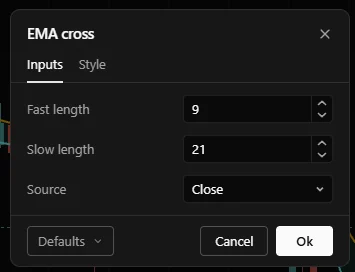
Opening the settings dialog
There are three ways in:
- The legend row. Each study on the chart has a row in the chart's legend, with buttons to hide the study, open its settings and remove it. A study written in OpenScript also has a braces button, which opens its source in the Scripts panel.
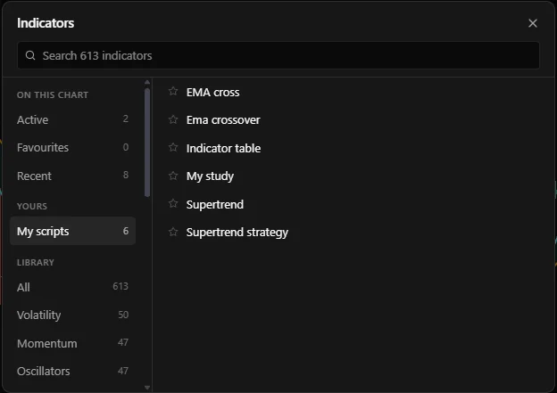
- The Indicators dialog. Under On this chart, Active lists every study on the chart, each with Settings and Remove.
- The Objects panel. On the right-hand toolbar, Objects lists what is on the chart, and each study there offers Hide, Settings and Remove.
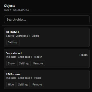
The dialog carries the study's title at the top, two tabs, Inputs and Style, and three buttons at the bottom: Defaults on the left, Cancel and Ok on the right.
- Ok applies what you changed and closes the dialog.
- Cancel, the close button, the Escape key or a click outside the dialog closes it without applying anything.
- Defaults puts the fields back to the script's defaults. Nothing is applied until you press Ok.
A tab with nothing on it is greyed out, so a study with no inputs opens straight on its Style tab.
The Inputs tab
The Inputs tab has one row per input() call, in the order they appear in the source, with the input's title as the label and a control chosen by the input's kind:
| Kind of input | Control |
|---|---|
| Number | A number box, with arrows that move by the input's step and stop at its min and max |
Switch (true or false) | A tick box |
Choice (options = [...]) | A menu of the listed values |
Source (close, hlc3 and so on) | A menu of Open, High, Low, Close, Hl2, Hlc3 and Ohlc4 |
Interval (kind = "interval") | A menu of Chart interval and the intervals your data feed serves |
| Colour | A colour swatch |
| Text | A text box |
Time (kind = "time") | A text box with the hint YYYY-MM-DD HH:MM, read as a UTC clock in /trading today |
The dialog does not show group headings or tooltips today, so write labels that say what a row is and in which unit. Inputs covers every kind, its bounds and the values it hands the script.
The Style tab
The Style tab has one row per plot(), labelled with the plot's title. You write none of it.
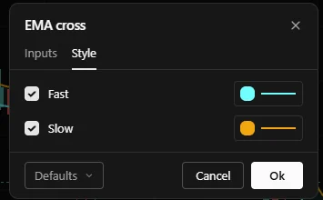
Each row has a tick box and an appearance button that shows the line's current colour and style. The tick box shows or hides that one plot: unticking it sets the plot's opacity to zero, and ticking it brings it back at full opacity. The appearance button opens a panel with:
- A palette of greys and colours. Picking one sets the colour and closes the panel.
- A plus sign, for any other colour from the browser's colour picker.
- Opacity, a slider from 0 to 100 percent.
- Thickness, one of 1, 2, 3 or 4 pixels.
- Line style: solid, dashed or dotted.
Two consequences save a script work.
A script never writes style for the reader's benefit. Write the colour and width that make the study readable on the day you ship it, and stop there. A trader who wants a thicker or dashed line changes it on the Style tab, and the change is kept. A script that tried to offer every option as an input would duplicate controls the reader already has.
Style is a preference, and a value is a computation. If a change affects a number, it belongs in an input. If it only affects how the same number looks, the Style tab already handles it.
What the Style tab does not offer in /trading:
- The plot's style. Whether a plot is a line, a step line, a histogram, columns or an area is decided by its
styleargument in the script. - Rows for anything but plots.
level(),fill(),background(),barColor()and tables have no Style rows. If a reader should be able to recolour one of those, give it a colour input, as the next section shows.
A colour with a meaning
Sometimes a colour carries meaning: the long side against the short side, one band against another. For those, declare a colour input and pass it to the plot.
version 1

study("Stop", overlay = true, precision = 2)

atrLen = input(10,  "ATR length", min = 1, max = 200)
mult   = input(3.0, "Stop distance, in ATR", min = 0.5, max = 20)

longTint  = input(lime, "Long stop colour",  group = "Colours")
shortTint = input(red,  "Short stop colour", group = "Colours")

atrValue = atr(atrLen)
var dir  = 1
var stop = none

prevStop = stop

if close > orElse(prevStop, low)
    dir = 1
else if close < orElse(prevStop, high)
    dir = -1

stop = dir == 1 ? hl2 - mult * atrValue : hl2 + mult * atrValue

// Two plots rather than one plot with a per-bar colour: each colour input is
// passed to a plot as it is, which makes it the same setting as that plot's
// Style colour, and the line breaks where the stop switches sides.
plot(dir ==  1 ? stop : none, "Stop, long",  longTint,  width = 2)
plot(dir == -1 ? stop : none, "Stop, short", shortTint, width = 2)
A colour input passed to a plot is the same setting as that plot's Style colour. The Inputs tab shows it under your title, "Long stop colour", and the Style tab shows it on the plot's row, and changing either changes both. So a reader never ends up with two colour controls for one line that disagree. This holds only when the input is passed as it is: a colour computed from an input, such as fade(longTint, 50) or up ? longTint : shortTint, is not tied to the Style row.
For a level or a shade, which have no Style row, a colour input is the only way to let the reader restyle it. Pass the input straight to the call:
version 1

study("Shaded range", overlay = true, precision = 2)

len       = input(20, "Lookback, in bars", min = 2, max = 500)
lineTint  = input(aqua,           "Range colour", group = "Colours")
shadeTint = input(fade(aqua, 90), "Shade colour", group = "Colours")
midTint   = input(gray,           "Midline colour", group = "Colours")

top    = highest(high, len)
bottom = lowest(low, len)

topPlot    = plot(top,    "Range high", lineTint, style = "step")
bottomPlot = plot(bottom, "Range low",  lineTint, style = "step")
fill(topPlot, bottomPlot, shadeTint)
level(0, "Zero", midTint)A colour that changes per bar
The colour argument of plot() takes either one colour or a colour that varies per bar. Pass an expression that varies, and the chart draws each bar in its own colour:
version 1

study("Momentum histogram", precision = 4)

upTint   = input(lime, "Rising colour")
downTint = input(red,  "Falling colour")

m = macd(close, 12, 26, 9)

level(0, "Zero", gray)

plot(m[0], "MACD",   aqua)
plot(m[1], "Signal", orange)
plot(m[2], "Histogram", m[2] > 0 ? upTint : downTint, style = "histogram")
When the script decides the colour on every bar, build that colour from colour inputs, as above, and the reader keeps control of both colours through rows you named. A per-bar colour built from bare colour names is one the reader cannot change at all.
Four helpers cover nearly every colour you need to build:
| Call | Does |
|---|---|
rgb() | Red, green and blue channels from 0 to 255, fully opaque |
rgba() | The same with an alpha from 0 to 1, where 1 is opaque |
fade() | The same colour at a given transparency in percent, where 100 is invisible |
withAlpha() | The same colour at a given opacity from 0 to 1 |
fade takes transparency and withAlpha takes opacity, and mixing them up draws something invisible. fade(aqua, 92) is the usual way to write a light shade. Colors has the rest.
Paint the reader did not ask for
background() and barColor() paint whole bars rather than drawing a plotted line, so they have no Style rows and the reader cannot turn them off there. Anything that paints over the reader's candles or the whole pane needs a switch of your own:
version 1

study("Session shading", overlay = true)

shade = input(true,  "Shade the opening minutes")
paint = input(false, "Recolour the candles")
tint  = input(aqua,  "Shade colour", group = "Colours")

opening = session.isIn("0915-0930", "Asia/Kolkata")

// An absent colour leaves the bar alone, which is how a paint switches itself
// off. It is not an error.
background(shade and opening ? fade(tint, 88) : none)
barColor(paint ? (close > open ? lime : red) : none)
Default a paint switch to false unless the study is about the paint. A study that recolours the instrument's candles the moment it is added has overwritten something the reader may have set up on purpose. Bar colouring and backgrounds has more.
What the declaration decides
The declaration is where a study says how it wants to be placed and formatted. Every option is fixed before the first bar, because the pane, the scale and the legend exist before any bar runs.
| Option | Type | Default | Decides |
|---|---|---|---|
title | string | required | The name on the legend row, in the Indicators dialog and at the top of the settings dialog |
short | string | the title | A shorter legend name, for a host that shows one. The /trading legend shows the full title |
overlay | bool | false | true draws on the price pane, false gives the study its own pane below the price |
precision | number | 4 | Decimals on the study's own pane, 0 to 10. A study drawn over the price keeps the instrument's own price formatting |
format | string | "price" | "price", "percent" or "volume" formatting on the study's pane |
range | array<number> | none | [min, max] to fix the study pane's scale, as in [0, 100] |
scale | string | "right" | "right", "left" or "none". The /trading chart places each line by the scale argument of its own plot(), so set it there |
group | string | "" | The category shown beside the study in the Indicators dialog. /trading shows OpenScript when you leave it empty |
onUnconfirmed | bool | false | Whether signals, alerts and orders may fire on a bar that is still forming. See Repainting |
In the Indicators dialog, every saved script that compiles is listed by its title under My scripts, and its group appears beside it when you point at the row.
version 1

study("Bounded oscillator", precision = 2, range = [0, 100], group = "Momentum")

len = input(14, "Length", min = 2, max = 200)

level(70, "Overbought", red)
level(50, "Middle", gray)
level(30, "Oversold", lime)

plot(rsi(close, len), "RSI", purple, width = 2)
range = [0, 100] is worth writing on any bounded oscillator. Without it the pane rescales to whatever the data did, so 70 stops meaning overbought and the reader compares a line against a moving frame. The range takes two numbers, lowest first:
version 1

study("Backwards", range = [100, 0])
plot(rsi(close, 14), "RSI")
precision belongs on the declaration and almost never on a plot. On a plot drawn over the price pane it would reformat the instrument's own price scale, which is rarely what anyone wants, and the compiler warns with OS8007:
version 1

study("Average", overlay = true)
plot(sma(close, 20), "Average", precision = 1)
The full list of options for study() and strategy() is in the declarations reference.
What /trading keeps
/trading keeps each chart's studies, with their settings, and brings them back when you return. What it keeps for a study:
| Kept | Filed under |
|---|---|
| The value of each input you changed | The input's key: the name it is assigned to, or its title when it has no name |
| Each Style change | The plot's position in the file: the first plot, the second plot, and so on |
| A colour input's value | The input's key, whichever tab you changed it on |
The study itself is tied to its script's file name, not to one version of the text. When you edit and save the script, the study keeps its saved settings.
Because values are filed by name and position, some edits reach the reader:
- Renaming an input's variable loses the reader's saved value for it, and the study comes back on the default. Renaming only its title keeps the value, unless the input is assigned to no name, because then the title is its key.
- Renaming a plot's title keeps its Style changes, because they are filed by position.
- Moving a plot above another, or deleting one before it, hands the saved Style changes to whichever plot now sits in that position.
- Tightening a bound can make a saved value invalid. The study then stops with OS6019, naming the setting and the rule it broke, rather than quietly using the default. Open the settings, correct the value or press Defaults, and press Ok.
Choose names and titles once, before anyone else loads the study, and treat a later rename as a change your readers will see.
Worked example: a study that gives away everything worth giving
version 1

study("Channel", overlay = true, precision = 2)

len = input(20,   "Length, in bars", min = 2, max = 500)
src = input(hlc3, "Source")

mult = input(2.0, "Width, in ATR", min = 0.2, max = 10, step = 0.1, group = "Channel")

showChannel = input(true,           "Show the channel", group = "Colours")
upperTint   = input(aqua,           "Upper colour",     group = "Colours")
lowerTint   = input(aqua,           "Lower colour",     group = "Colours")
basisTint   = input(orange,         "Basis colour",     group = "Colours")
shadeTint   = input(fade(aqua, 94), "Shade colour",     group = "Colours")

basis = ema(src, len)
band  = mult * atr(len)

// Computed on every bar; the switch hands the edge plots none to hide them,
// and the shade stops wherever its plots are absent.
upper = showChannel ? basis + band : none
lower = showChannel ? basis - band : none

plot(basis, "Basis", basisTint, width = 2)
upperPlot = plot(upper, "Upper", upperTint)
lowerPlot = plot(lower, "Lower", lowerTint)
fill(upperPlot, lowerPlot, shadeTint)
What the reader gets: three number and source rows, a switch and four colours on the Inputs tab, and on the Style tab a colour, opacity, thickness and line style for each of the three lines. What the script did not have to write: a single thickness input, a line style input, or any code to save and restore any of it.
Related: Inputs, Plots, Fills, Colors, Declarations reference, Repainting